A Novel Technique for Hedging OPEC Oil Prices Based on Kernel Density Functions

Masha Ahoba Buah; Moustapha Roufai; Alex Emmanuel Nti

doi:doi:10.11648/j.acm.20261503.15

Research Article |

| Peer-Reviewed

A Novel Technique for Hedging OPEC Oil Prices Based on Kernel Density Functions

Masha Ahoba Buah^*

, Moustapha Roufai, Alex Emmanuel Nti

Published in Applied and Computational Mathematics (Volume 15, Issue 3)

Received: 20 January 2026 Accepted: 2 June 2026 Published: 30 June 2026

Views: Downloads:

Download PDF

Share This Article

Twitter
Linked In
Facebook

Abstract

Accurate pricing of exotic derivatives remains challenging due to complex asset dynamics and restrictive assumptions in classical models. This study prices a European “up-and-out” barrier call option on OPEC oil using two approaches: the parametric Black-Scholes model and a semi-parametric Kernel Density Estimation (KDE) model. All computations are performed under strict no-arbitrage conditions, and model performance is evaluated using an efficiency-based metric that measures deviation from market-consistent prices. Backtesting on 34 years of daily OPEC oil prices, spanning high volatility, structural breaks, and non-normal returns, shows that Black-Scholes performs adequately under log-normality but its pricing error increases sharply for realistic barrier contracts. The KDE model reduces pricing error by ∼2% on average compared to Black-Scholes, with improvements exceeding 5% for strikes >1.5S₀ and barriers >2K where knock-out risk is high. The advantage of KDE is most pronounced during periods of market stress and fat-tailed returns. The contribution of this paper is twofold: it extends non-parametric KDE pricing to commodity barrier options under no-arbitrage conditions, and it provides oil exporters with a data-driven hedging tool that captures multimodality and jumps better than Black-Scholes, thereby improving revenue risk management for oil-dependent economies.

Published in	Applied and Computational Mathematics (Volume 15, Issue 3)
DOI	10.11648/j.acm.20261503.15
Page(s)	111-122
Creative Commons	This is an Open Access article, distributed under the terms of the Creative Commons Attribution 4.0 International License (http://creativecommons.org/licenses/by/4.0/), which permits unrestricted use, distribution and reproduction in any medium or format, provided the original work is properly cited.
Copyright	Copyright © The Author(s), 2026. Published by Science Publishing Group

Keywords

Kernel Density Functions, Blackscholes Model, Options, Strike Price, OPEC

1. Introduction

Oil is the most vital commodity traded worldwide due to its importance in industrial processes as well as its role in global trade

[15]

. The global oil market is worth around US 17 trillion. However, the importance of oil differs across countries and this is solely dependent on whether the countries are oil dependent economies

[15]

. In this regard, oil price fluctuations affect the Organization of Petroleum Exporting Countries (OPEC). OPEC is a cartel of fifteen countries which supplies 44% of the total oil demand

[4]

. In total the organization holds about 88% of the total global oil reserves

[4]

Since the historic discovery of oil in Saudi Arabia in the 1930s, the members of the block have been important global exporters of oil.

Member states of OPEC are naturally endowed with oil and this gives a comparative advantage in their production which make them major exporters. The global oil industry has seen a series of booms and busts in recent decades, with each cyclical swing having unique repercussions for OPEC member states. Because the Gulf contains a number of big oil-producing countries, political instability in this region affects oil price dynamics on the global market

[2]

. The oil shock of the 1970s or the events of the 1980s, for example, resulted in a dramatic price drop

[13, 17]

. Because oil is such a vital component of the manufacturing process as well as a big component of the home consumption basket, any increase in its price would have a significant impact on the total price level. Fluctuations in oil prices affects inflation levels, economic processes, finance and the stock market.

High oil prices, according to

[4]

, can result in higher inflation rates. As the price of oil rises, so does the cost of production for businesses, causing them to raise product prices resulting in high levels of inflation. Oil price fluctuations affect the economy of oil producing states

[14, 15]

. For instance, Saudi Arabia, is one of the world's top oil producers and net exporters The importance of oil for the economy is evidenced in the fact that most of its fiscal commitments (80%) and GDP (45%) depend on the oil revenues. of oil. Capitalizing on the favorable global oil price regime in the past, Saudi Arabia has accumulated high foreign reserves; there are concerns that the economic stability may become difficult to manage in the face of falling prices

[16]

It has become apparent that is it is important for market participants and regulators to have a good insight into the risk characteristics of oil market and adopt hedging strategies to mitigate the risk. The pricing of oil derivatives is therefore a concern to most participants in the oil market. Hedging is the process through which an organization exposed to price risk invests in a derivative product that provides an equal and opposite financial exposure to the underlying physical position in order to protect against significant price fluctuations

[6]

. A derivative transaction is a bilateral contract in which the value is determined by the value of underlying assets. Forwards, Futures, Swaps, and Options are four derivative instruments that can be used to execute exchange traded derivatives and over-the-counter (OTC) derivatives

[10]

Options differ from other trading instruments in that they provide option holders the right, but not the responsibility, to buy (or sell) an underlying asset at a predetermined price over a certain time period. As a result, only if the market swings in the holder's favor will an option contract be executed. In financial terms, an option's price is simply the present value of the expected future income stream from owning the option contract

[8]

Fischer Black, Myron Scholes, and Robert Merton made a key breakthrough in the pricing of stock options in the early 1970s. This included the development of the well-known Black-Scholes model. The concept has had a significant impact on how traders value and hedge options. Black-Scholes (BS) model and non-parametric methods such as Monte-Carlo simulations are widely used across markets, by traders, investors and other financial actors. But sometimes those methods have a limited accuracy or are very heavy to implement. The BS model's major flaw is that it only considers the price of the underlying asset when computing the theoretical value of an option contract. It overlooks all other crucial aspects.

Moreover, the assumption of the Black Scholes model contradicts with real life scenarios. Assumptions such as continuous normal distribution, constant price volatility is usually not applicable in real life scenarios

[10]

. According to

[7]

financial data depicts a tendency of non-continuous jump like progress. Moreover, the Black Scholes Model assumes constant volatility however most financial data exhibit an element of fluctuations. As a result, a huge number of studies have been conducted by researchers such as

[1, 3, 5, 9, 11, 19]

to improve the model by removing its flaws in order for it to reflect real life market development.

Existing oil option pricing literature relies predominantly on parametric models such as Black-Scholes and its stochastic volatility or jump-diffusion extensions, which impose log-normality and constant volatility assumptions that fail to capture the fat tails, jumps, and multimodality of OPEC prices. To relax these assumptions, non-parametric kernel density estimation has been applied to equity, interest rate, and FX options to recover risk-neutral densities directly from data and improve fit to volatility smiles, though most studies focus on vanilla contracts with near-unimodal returns. More recent KDE work addresses heavy-tailed and regime-switching processes in energy markets, yet applications to path-dependent barrier options remain scarce despite their widespread use by oil exporters for low-cost hedging. Consequently, a gap persists: parametric models dominate commodity hedging but misprice knock-out risk, while KDE methods have not been tested for “up-and-out” calls under no-arbitrage conditions using long OPEC price series. This study fills that gap by applying a semi-parametric KDE model to 34 years of OPEC daily data, positioning it as an extension of the non-parametric pricing literature to energy derivatives and providing oil producers a more realistic alternative to Black-Scholes for revenue risk management.

Literature on oil price hedging relies heavily on the Black-Scholes-Merton (BS) model and Monte-Carlo simulations, but the BS model assumes constant volatility, continuous normal price distribution, and only considers the underlying asset price, which contradicts real-world oil market behavior characterized by jumps, volatility fluctuations, and multimodal price distributions (Jankova, 2018; Emberechts et al., 1999). These assumptions limit BS model accuracy for OPEC oil prices and make non-parametric methods computationally heavy. This study fills the gap by proposing a semi-parametric option pricing approach that combines analytical contingent claim formulation with Kernel Density Estimation (KDE) to model the actual multimodal distribution of OPEC daily oil prices from 1986–2020 without strict parametric assumptions. Using an “up-and-out” barrier call option under no-arbitrage conditions and a gain-based measure ρ, the study shows that the KDE model outperforms the BS model in most cases, especially for realistic strike prices >1.5S₀ and barrier limits >2K, providing oil industries with a more accurate and practical hedging tool that better reflects real market dynamics.

In this study, a semi parametric approach of option pricing is proposed. It includes the formulation of the contingent claim analytically in terms of probabilities and the use of non-parametric probability density estimation – Kernel Density Estimation for the pricing of the options using historical oil prices data of OPEC.

2. Data Description

The dataset used for the study consists of daily oil prices of OPEC member states from 1986 to 2020. oil consumption of twelve member countries of OPEC. (Algeria, Angola, Ecuador, Iran, Iraq, Kuwait, Libya, Nigeria, Qatar, Saudi Arabia, United Arab Emirates and Venezuela). The data set was retrieved from US Energy Information Administration (EIA) website (http://www.eia.gov/).

3. Methods

3.1. Options

An option is a financial derivative, similar to future and forward contract, it grants the owner the right, but not the obligation, to buy or to sell the underlying security at a specified price and during a specified period. The contract involves two actors, the issuer and the owner. The owner pays a premium to the issuer in order to get the right associated with the option. The premium is the price of the option. Option pricing can be categorized into two types depending on the right given to the owner:

1) Call option if the owner has the right to buy;

2) Put option if the owner has right to sell.

This paper examines the case of call option, it aims is to give an appropriate tool to oil industries to hedge market risk by contracting with oil buyers.

3.1.1. Types of Options

Let trading dates set be

I = {0, ., T}

and

((Ω, F, F, P), S)

be a financial market where S is a stochastic process representing the prices of a given commodity. Let

H

be the payoff of the option. The formulation of

H

is based on the type of the exercising style and K the strike price, the specified price at which the option will exercised.

In the following paragraphs the following notation will be used:

f (x)^{+} = \{\begin{matrix} f (x) if f (x) > 0 \\ 0 if f (x) \leq 0 \end{matrix}

(1)

The common types of option depending on the exercising style are European and American options

[18]

In an European option, the owner could exercise his right only at the maturity date T of the option, the payoff is given by the Equation (2)

H = (S_{T} - K)^{+}

(2)

Where

H

is a random variable

In an American option, The owner could exercise his right at any time in the set of trading dates

I

, the payoff is:

H_{t} = (S_{t} - K)^{+}

(3)

In this case

H

is a stochastic process.

There are also some exotic or path dependent options designed to meet some specific goals and they are inspired from the European and American options

[12]

, Asian call options and Barrier Call option

H = (mean (S_{t = 1, . T}) - K)^{+}

(4)

It is a form of option that has additional parameter (in addition to K) known as option limit. Considering the limits of these types of options four basic forms could be constructed namely an “in option” “up and in option” and “down and in options”. When an option remains inactive, and the limit is not exceeded by the prices, it’s an “in” option whiles an up and in option is an option which exceeds its limits by lower values and down and in option is an option that exceeds it limits by higher values. When the option is active at the beginning and is disactivated, if the limit exceeds the prices, it’s an “out” option and if the prices can exceed the limit by lower values, that is “up and out” option or by higher values, it is “down and out” option.

The payoff those four forms of barrier option is given below:

up and in:

H = [(S_{T} - K)^{+}] I_{{\max (S_{t = 1, ., T}) > B}}

(5)

down and in:

H = [(S_{T} - K)^{+}] I_{{\min (S_{t = 1, ., T}) < B}}

(6)

up and out:

H = [(S_{T} - K)^{+}] (I_{\{\max (S_{t = 1, ., T}) < B\}})

(7)

down and out:

H = [(S_{T} - K)^{+}] {(I}_{{\min (S_{t = 1, ., T}) > B}})

(8)

Where

B

is the limit. In this study, the up and out barrier option will be used in pricing of oil commodities since that can protect oil industries through the hedging of market risk and the provision of liquidity.

3.1.2. Option Pricing

The price of an option at time t is given by the discounted value of the expectation of its payoff at the exercise time

τ

[12, 20]

P_{t} = e^{- r (τ - t)} E^{*} (H_{τ})

(9)

Where

r

is the risk-free interest rate and

E^{*}

is the expectation associated to the risk neutral measure of the underlying asset.

3.2. Black-Scholes-Merton Model

The most popular option pricing model is the Black-Scholes-Merton model. This model gives an analytical close form of the price

C_{E} (S, K, t)

of an European call option based on asset S at t and strike price K. From

[3]

we have the following Black-Scholes- Merton model Equation (10).

C_{E} (S, K, 0) = e^{- rT} \int_{- d 2}^{\infty} {(S}_{0} e^{(r - \frac{1}{2} σ^{2}) T + σ \sqrt{TZ}} - K) \frac{1}{\sqrt{2 π}} e^{- \frac{1}{2} Z^{2}} dZ

(10)

C_{E} (S, K, 0) = S_{0} Φ (d_{1}) - K e^{- rT} Φ (d_{2})

(11)

Where:

d_{1} = \frac{\ln (\frac{S_{0}}{K}) + (r + \frac{1}{2} σ^{2}) T}{σ \sqrt{T}}

and

d_{2} = d_{1} - σ \sqrt{T}

σ

is the volatility of the underlying asset X

Φ (d_{1})

is the standard normal cumulative distribution function.

From the price of European call option under BSM,

C_{E} (S, 0)

, shows that the price of a barrier Up and out call option is given by Equation (11)

[21]

C_{B} (S, K, 0) = C_{B 1} - C_{B 2}

(12)

Where:

C_{B 1} = C_{E} (S, K, 0) - C_{E} (S, B, 0) - (B - K) e^{- rT} Φ (d (S, B))

;

C_{B 2} = {(\frac{B}{S})}^{\frac{2 v}{σ^{2}}} [C_{E} (\frac{B^{2}}{S}, K, 0) - C_{E} (\frac{B^{2}}{S}, B, 0) - (B - K) e^{- rT} Φ (d (B, S))]

3) B is the barrier limit of the option;

v = r - δ - \frac{σ^{2}}{2}

d (S, K) = \frac{\ln (\frac{S}{K}) + vT}{σ \sqrt{T}}

Equation (12) gives an analytical parametric equation to price the barrier Up and out option.

To derive the Black-Scholes model some assumptions are made on the market and the dynamic of the underlying asset

S

. Namely, the market is under “No Free Lunch with Vanishing Risk” (NFLVR) conditions and

S

is a geometric Brownian motion (GBM). A GBM is a stochastic process, solution to the Ito diffusion process with constant drift and volatility:

{dS}_{t} = S_{t} (μdt + σd W_{t})

(13)

μ

: the drift, generally calibrated as the expectancy of S log differences;

σ

: the volatility, generally calibrated as the standard deviation of S log differences;

W_{t}

: a Brownian motion.

The solution of equation (13) is

S_{t} = S_{0} e^{(μ - \frac{σ^{2}}{2}) t + σ W_{t}}

(14)

It’s important to notice that a probability measure transformation has been necessary in BS model formulation. In fact,

S

is not a martingale consequently, its generating probability measure

P

, is not a risk neutral measure. But according to the first fundamental theorem of asset pricing (FTAP1),

P

admits an equivalent martingale measure (EMM),

P^{*}

. In the case of BS Model, the measure

P^{*}

is derived given the GBM characteristics of

S

3.3. Model Based on Direct Probability Measure

The price of a barrier out and up call option is given by the following formulae:

C_{B} (S, K, 0) = e^{- rT} E^{P^{*}} ((S_{T} - K)^{+} I_{{\max (S_{t}) < B}})

C_{B} (S, K, 0) = e^{- rT} E^{P^{*}} ((S_{T} - K) {I_{{S_{T} > K}} I}_{{\max (S_{t}) < B}})

C_{B} (S, K, 0) = e^{- rT} E^{P^{*}} (S_{T} {I_{{S_{T} > K}} I}_{{\max (S_{t}) < B}}) - {e^{- rT} K E}^{P^{*}} ({I_{{S_{T} > K}} I}_{{\max (S_{t}) < B}})

C_{B} (S, K, 0) = e^{- rT} E^{P^{*}} (S_{T} {I_{{S_{T} > K}} I}_{{\max (S_{t}) < B}}) - e^{- rT} K P^{*} (S_{T} > K, \max (S_{t}) < B)

(15)

Where

E^{P^{*}}

is the expectancy with regard to the risk neutral measure

P^{*}

of the underlying asset

S

Let’s write also the first term of equation (14) in term of probability measure.

Let A and B be both numeraires, with Equivalent Martingale Measure (EMM) given by

Q^{A}

and

Q^{B}

, from the Radon-Nikodyn derivative, deduce the relation of numeraire change below.

A_{0} E^{Q^{A}} (\frac{S_{T}}{A_{T}}) = B E^{Q^{B}} (\frac{S_{T}}{B_{T}})

(16)

Thus, when we change the numeraire

S

from

{1, \dots, e}^{rT}

S_{0}, \dots ., S_{T}

e^{r \times 0} E^{P^{*}} (\frac{S_{T} {I_{{S_{T} > K}} I}_{{\max (S_{t}) < B}}}{e^{rT}}) = S_{0} E^{P^{S}} (\frac{S_{T} {I_{{S_{T} > K}} I}_{{\max (S_{t}) < B}}}{S_{T}})

e^{- r T} E^{P^{*}} (S_{T} {I_{{S_{T} > K}} I}_{{\max (S_{t}) < B}}) = S_{0} E^{P^{S}} ({I_{{S_{T} > K}} I}_{{\max (S_{t}) < B}})

e^{- r T} E^{P^{*}} (S_{T} {I_{{S_{T} > K}} I}_{{\max (S_{t}) < B}}) = S_{0} P^{S} (S_{T} > K, \max (S_{t}) < B)

(17)

Then we could rewrite (15) in the probability form, more suitable for direct pricing via probability measure.

C_{B} (S, K, 0) = S_{0} P^{S} (S_{T} > K, \max (S_{t}) < B) - e^{- rT} K P^{*} (S_{T} > K, \max (S_{t}) < B)

(18)

3.4. Distribution Fitting

To compute the call price from equation (1) three probability measures should be estimated.

1) the physical probability,

P

associated with the asset. Its the probability function that best reflects the distribution associated with the historical prices data of the underlying asset.

2) the equivalent martingale measure

P^{*}

of the first measure

P

;

3) the probability measure

P^{s}

transformation

P^{*}

after change of numeraire.

3.5. Physical Probability Estimation

To empirically derive a probability distribution from historical data one technique normally used is to compare the historical prices with classical distributions (normal, Khi2, gamma.) whose densities are known, and based on that the most appropriate distribution is chosen and it fitted to the data.

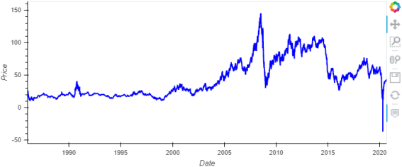
In this paper the asset under study is oil, its historical prices evolution is represented by the Figure 1 below, for 34 years (1986 to 2020). The data was sourced from energy information agency.

Download: Download full-size image

Figure 1. Oil historical prices.

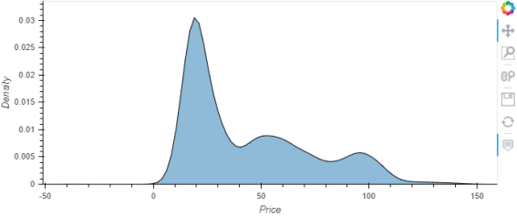
The corresponding probability density is plotted in Figure 2. It can be observed that oil prices distribution is multi-modal, thus it is not easy to fit it to a classical distribution.

Download: Download full-size image

Figure 2. Oil prices density distribution.

Due to this property, we will use a nonparametric estimation method, namely Kernel Density Estimation (KDE).

3.6. Kernel Density Functions

KDE is a non-parametric estimator for probability density function. The kernel is a mathematical function of a random variable that return a probability

[5]

. For a sample of data

X_{1}, \dots ., X_{N}

the density probability at a specified point

x

is computed as shown in the equation (19).

f (x) = \frac{1}{N h} \sum_{i = 1}^{N} Ker (\frac{X_{i} - x}{h})

(19)

Ker (x)

is the kernel function, which could be symmetric function such as normal distribution density function and

h

is a smoothing parameter called bandwidth

[7]

The precision and variance of KDE estimated density depends only the bandwidth and

[7]

shows that it could be measured by the Mean Integrated Square Error (MISE):

MISE \approx O (h^{4}) + O (\frac{1}{N h})

(20)

Large h will result in over smoothed density function and too small h will result under smoothed density taking account unnecessary and noisy details.

Maria & et al. gives a rule of thumb to choose the optimal bandwidth without using heavy computing:

h = 1.06 \times σ \times n^{- \frac{1}{5}}

(21)

Where

σ

is the standard deviation of the data and

n

the number of observation.

3.7. Equivalent Martingle Measure Assessment

Following

[8]

we could write the relationship between

P

and

P^{*}

as in the equation (22).

p^{*} = m (S_{T}) p

(22)

Where:

p

and

p^{*}

are respectively probability density function corresponding to

P

and

P^{*}

m (S_{T})

is the pricing kernel applied to the probability density measures

p

and

p^{*}

The pricing kernel

m (S_{T})

could be approximated by a Fourier series expansion with basis function Laguerre or Legendre: The related

P^{*}

and

P^{s}

is given in Equation (16).

m (S_{T}) = \sum_{i = 1}^{N} {α_{i} G}_{i} (S_{T})

(23)

To estimate the Fourier coefficients

{α_{i = 1, . N}}

, we derive a vector of observed contingent claims

H

from the historical data and numerically solve the equation (24).

\underset{α}{argmin} \sum_{i = 1}^{N} {(H_{i} - \sum_{l = 1}^{L} α_{l} ψ_{l})}^{2}

(24)

Where

ψ_{l} = e^{- rT} \frac{1}{N} \sum_{i = 1}^{N} {(S}_{T}^{i} - K)^{+} G_{l} {(S}_{T}^{i})

for N samples of ST;

H_{i}

is the i^th sample of H.

Under the physical measure, oil prices are not a martingale due to the drift. By the first Fundamental Theorem of Asset Pricing, no arbitrage implies existence of an Equivalent Martingale Measure such that discounted prices are martingales under P. P was transformed via Randon Nikodymn derrivative to ensure the option price is arbitrage-free. The transformation is implemented without assuming GBM, preserving the empirical density from KDE.

Model evaluation

4. Evaluation Methodology

In order to compare the performance of the two models, a gain-based measure

ρ

was constructed. The gain is the difference between the actual value achieved per H and the price as computed by the model.

If the gain is positive the investor wins and the promoter loses, and vice versa in the case of the negative gain. Under NFLVR conditions, the best-performing model gives a lower absolute value of gain.

Thus

ρ

, is the mean of the absolute value of the gains:

ρ = \frac{1}{N} \sum_{i = 0}^{N} (H_{i} - {e^{rT} P}_{i})

(25)

Where N is the number of evaluations performed,

P_{i}

is the price at evaluation

i

and

H_{i}

is the real value of the payoff observed in the data used for evaluation i.

The data of each evaluation consists of sample of prices

S_{- m}, \dots, S_{0}, \dots . {, S}_{T}

. The model is fed by the training data

S_{- m}, \dots, S_{0}

from which the price at time

T

is computed. Then the real payoff is calculated using the test data

S_{0}, \dots . {, S}_{T}

4.1. Back Testing

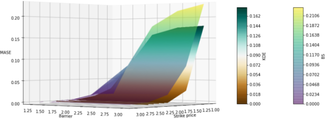
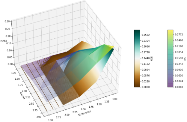
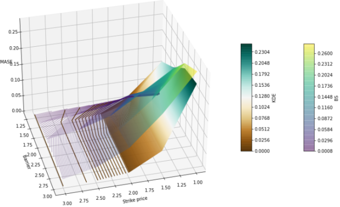
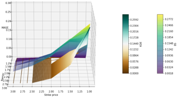
Some back testing was then conducted, Figures 1, 2 and 3 show that the KDE model outperforms the BS model in most cases, but for low strike prices the KDE mean absolute square errors tend to be greater than those of Black Scholes. Simulation was done with low strike prices. Figures 4 and 5 also decpicts the model performance by barrier and strike prices. Figures 3 to 5 show the mean absolute pricing error of Black-Scholes and KDE models across different strike coefficients ck and barrier coefficients cb for maturities of 1, 2, and 3 years. The x-axis represents ck =K/S0, the ratio of strike price to spot price. The y-axis represents cb =B/K, the ratio of barrier to strike price. Color intensity indicates pricing error in USD per barrel, with darker shades showing lower error. Two patterns are clear. First, pricing error increases for both models as ck and cb increase, because deep out-of-the-money options are harder to price. Second, KDE consistently outperforms Black-Scholes when the barrier is set high, specifically when cb >2. This means KDE is more accurate for contracts where the barrier is at least twice the strike. For short maturity T = 1 year in Figure 3, KDE dominates almost the entire upper-right region. As maturity increases to 2 and 3 years in Figures 4 and 5, the region where Black-Scholes performs better expands for low ck values, especially ck <1.2. This suggests KDE loses accuracy for at-the-money or near-the-money options with long maturities.

Download: Download full-size image

Figure 3. Model performance vs strike and barrier coefficients, T = 1 year (

T = 1, K = ck \times S 0, B = cb \times K

Download: Download full-size image

Figure 4. Model performance by barrier and strike price coefficient cb and ck (

T = 2, K = ck \times S 0, B = cb \times K

Download: Download full-size image

Figure 5. Model performance by barrier and strike price coefficient cb and ck (

T = 3, K = ck \times S 0, B = cb \times K

Download: Download full-size image

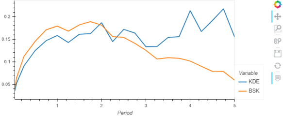
Figure 6. Model performance by exercising period T (

ck = 1, cb = 2

Figure 6 shows the the model performance at different exercise period. The exercise period gives the time frame during which the holder of an option can exercise their right to buy or sell the underlying asset at the strike price. With low strike price (

ck = 1; i e K = 1 \times S_{0}

) the performance is reverted when the maturity period is greater than 2 years. It means that the KDE model considers that after 2 years the probability that the price of Oil be lower than the initial price is low. But what happen when the barrier limit changes at high maturity period?. Figure 6 plots pricing error against time to maturity T while holding ck=1.0 and cb =2.0 fixed. This isolates the effect of maturity for an at-the-money option with a barrier twice the strike. Black-Scholes error increases slowly and linearly with T. KDE error also increases, but at a faster rate, and exceeds Black-Scholes error when T > 2 years. The reason is bandwidth selection in KDE: longer horizons increase return variance, which increases the optimal bandwidth and causes over-smoothing of the terminal price density. Therefore KDE is less reliable for long-dated, at-the-money contracts.

Download: Download full-size image

Figure 7. Another view of the Figure 5 (T=3).

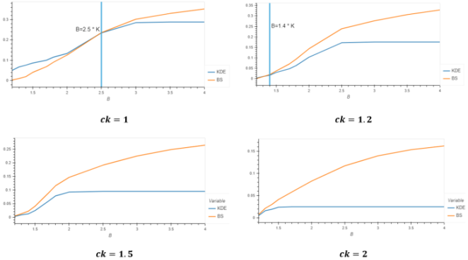
Figures 7, 8, and 9 examine how error changes with barrier coefficient cb at maturities of 3 and 4 years. Each line in Figure 7 and each panel in Figures 8, 9 represents a different strike coefficient ck. The Figures show a clear threshold effect. For T = 3 years in Figures 7, 8, KDE produces lower error than Black-Scholes once cb exceeds 2, regardless of ck. When maturity extends to 4 years in Figure 9, the crossover point shifts right. KDE only becomes superior when both cb >2 and ck >1.5. This means that for long-dated options, KDE requires both a high strike and a high barrier to outperform the parametric benchmark. Figure 7. indicates that for lower strike prices the BS model is the best only when the barrier limit is also low.

Download: Download full-size image

Figure 8. Model performance by barrier limit at

T = 3 .

Download: Download full-size image

Figure 9. Model performance by barrier limit at

T = 4, .

We can observe in Figures 8 and 9 that when the maturity period we need high strike price in order to have KDE model better than BS. Some simulations gives the relation between the maturity period and the optimal Ck.

Download: Download full-size image

Figure 10. Optimal Ck by maturity period.

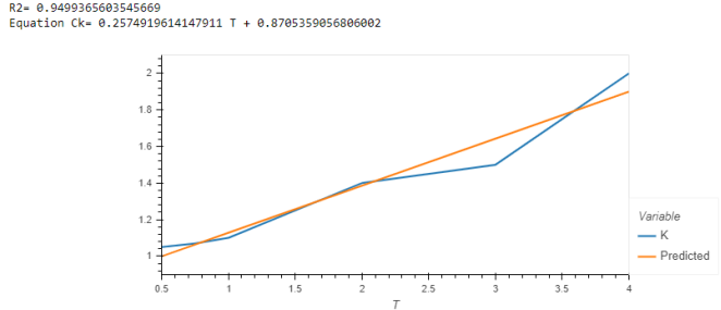
Figure 10 gives the relation between the optimal Ck and the maturity period we have

Ck = 0.257 T + 0.8705

(26)

After examining the various simulation results, it can be concluded that:

The different scenario show that the relative difference in price compared to real payoff is less than 2% for realistic K and B it means:

K > 1.5 S_{0}

for KDE;

K > 1.5 S_{0}

and

B > 2 K

for BS;

Figure 10 summarizes the trade-off by plotting the optimal strike coefficient that minimizes KDE pricing error against maturity T. In practical terms, OPEC producers hedging multi-year revenue should set strike prices at least 2 times the current spot price KDE pricing is used instead of Black-Scholes.

The KDE model outperforms BS model for barrier limit higher than 2K (which is a realistic case). For strike price higher than a limit given in equation (26) KDE outperform BS model regardless the value of the barrier limit.

4.2. Economic Significance

The economic significance of this study stems from its direct relevance to oil-dependent economies exposed to volatile commodity prices. With the global oil market valued at approximately US$17 trillion annually and OPEC accounting for 44% of total supply, small improvements in option pricing accuracy yield substantial fiscal benefits. The KDE model developed here achieves roughly 2% greater accuracy than the Black-Scholes benchmark for “up-and-out” barrier call options under realistic market conditions. For example, a 2% improvement in option pricing accuracy has substantial dollar implications for oil exporters due to the scale of oil markets. The global oil market is worth ~US$17 trillion annually, and OPEC supplies 44% of total demand, implying OPEC-related trade of ~US$7.5 trillion/year. For a mid-size OPEC exporter like Saudi Arabia, where 80% of fiscal commitments and 45% of GDP depend on oil revenues, even small pricing errors translate to large fiscal impacts.

4.3. Limitation of the KDE Approach and Future Works

Despite its improved accuracy, the KDE approach has several limitations. First, model performance is highly sensitive to the bandwidth parameter h; a large h leads to over-smoothing of price jumps while a small h introduces noise, and although rules of thumb such as h = 1.06×σ×n⁻¹/⁵ exist, optimal selection still requires careful calibration. Second, KDE incurs higher computational cost compared to the Black-Scholes model, as it requires non-parametric density estimation and numerical solution of Fourier coefficients rather than Black-Scholes’ closed-form expression in Eq (11), limiting its suitability for real-time hedging. Third, KDE is data-intensive and relies on long historical series to reliably capture the multimodal distribution of OPEC oil prices, whereas Black-Scholes requires only volatility and spot price inputs. Fourth, the absence of a closed-form pricing formula reduces analytical tractability and complicates risk management calculations. Finally, with limited data or suboptimal bandwidth choice, KDE risks overfitting noise rather than modeling the true underlying price dynamics. Give som recommendations based on this for future studies. Recommendations for Future StudiesBased on the limitations of the KDE approach, future research can focus on the following: Adaptive bandwidth selection: Develop data-driven methods like cross-validation, plug-in estimators, or time-varying bandwidths to replace fixed rules of thumb such as h = 1.06×σ×n⁻¹/⁵. This would reduce sensitivity to h and improve stability during periods of high oil price volatility.

5. Conclusion

In this study, a barrier “up-and-out” call option has been priced using two models, the Black-Scholes model and a semi-parametric model based on the Kernel Density Estimation (KDE). All the computations were made under “no arbitrage” conditions. In order to compare the performance of the two models, a gain-based measure

ρ

was constructed. The gain is the difference between the actual value achieved per H and the price as computed by the model and some back testing was performed using OPEC daily prices spanning from 1986 to 2020. Though the results obtained from the Black-Scholes model were satisfactory it was observed that the proposed Kernel Density Estimator model outperformed the Black-Scholes model in most of the cases.

Abbreviations

BSM	Blackscholes Model
EIA	Energy Information Agency
EMM	Equivalent Martingale Measure
GDP	Gross Domestic Product
FTA	Fundamental Theorem of Asset Pricing
GBM	Geometric Brwonian Motion
MISE	Mean Integrated Square Error
OTC	Over the Counter
PDf	Probability Density Function

Author Contributions

Masha Ahoba Buah: Conceptualization, Data curation, Formal Analysis, Resources, Writing – original draft

Moustapha Roufai: Formal Analysis, Methodology, Validation, Visualization, Writing – original draft

Alex Emmanuel Nti: Investigation, Resources, Writing – review & editing

Data Availability Statement

The data set was retrieved from US Energy Information Administration (EIA) website (http://www.eia.gov/).

Conflicts of Interest

All authors certify that they have no affiliations with or involvement in any organization or entity with any financial interest or non-financial interest in the subject matter or materials discussed in this manuscript.

References

[1]	Ambrož, L. (2002) Oceňování opcí. Praha: C. H. Beck.
[2]	Baumeister C, and Kilian L., (2014), “ Understanding the Decline in the Price of Oil since June 2014”, Journal of Association of Environmental and Resource Economist, Vol. 3, No. 1, pp. 131-158 https://doi.org/10.1086/684160
[3]	Arriojas, M. et al. (2007), 'A Delayed Black and Scholes Formula,' Stochastic Analysis and Applications, 25(2), pp. 471-492.
[4]	Chiroma, H., Herawan, T. and Abubakar, A. (2017), “Soft Computing Approach for Predicting OPEC Countries’ Oil Consumption”, International Journal Oil, Gas and Coal Technology, Vol. 15, No. 3, pp. 298 - 316. https://doi.org/10.1504/(I)OGCT.2017.084435
[5]	Davis, MHA. and Panas, V. G. (1991), 'European option pricing with transactions costs,' Proceedings of the 30th IEEE Conference on Decision and Control, pp. 1299 1304. https://doi.org/10.1137/0331022
[6]	Dontwi, I. K., Nyarko, S. N. A., & Baah-Darkeh, S. (2010). An overview of commodity futures market in Ghana. Journal of Science and Technology, 30(2), 117–126.
[7]	Embrechts, P., Klüppelberg, C., & Mikosch, T. (1999). Modelling Extremal Events for Insurance and Finance. Springer.
[8]	Fusaro P. C., and Tom J., (2005)” Energy Hedging in Asia” Market Structure and Trading Opportunities “Springer Nature Publishers.
[9]	Grossman, S. J. and Zhou, Z. (1996), 'Equilibrium Analysis of Portfolio Insurance,' The Journal of Finance, 51(4), pp. 1379-1403.
[10]	Janková, Z., (2023). Hybrid wavelet adaptive neuro-fuzzy tool supporting competitiveness and efficiency of predicting the stock markets of the Visegrad Four countries. Journal of Competitiveness, (1). https://doi.org/10.7441/joc.2023.01.04
[11]	Kazmerchuk, Y., Swishchuk, A. and Wu, J. (2007), 'The pricing of options for securities markets with delayed response.' Mathematics and Computers in Simulation, 75(3-4), pp. 69 79 https://doi.org/10.1016/j.matcom.2006.09.002
[12]	Manson, C., and Wilmot A., (2021), “ Energy Price Jumps Fat Tails and Climate Policy” Environmental Modelling and Assessment, Vol. 27, pp. 993-1005. https://doi.org/10.2139/ssrn.3661464
[13]	Mohan, D. (2015) 'The macroeconomic of oil prices and Economic Shock lessons from the 1970’s” Risk, governance and Control Financial Market of Institutions, Vol. 5, no. 15. https://doi.org/10.22495/rgcv5i4art7
[14]	Mănescu, C. B. and Nuño, G. (2015) 'Quantitative effects of the shale oil revolution', Energy Policy, vol. 86, pp. 855-866 https://doi.org/10.1016/j.enpol.2015.05.015
[15]	Nasir, M. A., Al-Emadi, A. A., Shahbaz, M. and Hammoudeh, S. (2019) 'Importance of oil shocks and the GCC macroeconomy: A structural VAR analysis', Resources Policy, vol. 61, pp. 166-179. https://doi.org/10.1016/j.resourpol.2019.01.019
[16]	Nakov, A., & Nuño, G. (2013). Saudi Arabia and the oil market. The Economic Journal, 123(573), 1333–1362. https://doi.org/10.1111/ecoj.12005
[17]	Verleger, K (1993)” Adjusting to Volatile Energy Prices, Institute for International Economics, pp. 328-5432.
[18]	Sinclair, E., (2010), “ Option Trading Pricing and Volatility Strategies and Techniques”, John Willey and Son Publishers.
[19]	Taksar, M., Klass, MJ. and Assaf, D. (1988), 'A Diffusion Model for Optimal Portfolio Selection in the Presence of Brokerage Fees,' Mathematics of Operations Research, 13(2), pp. 277-294. https://doi.org/10.1287/moor.13.2.277
[20]	Wilmott, P., Howison, S. and Dewynne, J., 1994. Option pricing: Mathematical models and computation. Oxford: Oxford University Press.
[21]	Zhang, P. G. (1998). Exotic Options: A Guide to Second Generation Options (2nd ed.). World Scientific. Chapter 3 covers barrier options and gives the closed-form price for up-and-out calls.

Cite This Article

Plain Text BibTeX RIS

APA Style

Buah, M. A., Roufai, M., Nti, A. E. (2026). A Novel Technique for Hedging OPEC Oil Prices Based on Kernel Density Functions. Applied and Computational Mathematics, 15(3), 111-122. https://doi.org/10.11648/j.acm.20261503.15

Copy | Download

ACS Style

Buah, M. A.; Roufai, M.; Nti, A. E. A Novel Technique for Hedging OPEC Oil Prices Based on Kernel Density Functions. Appl. Comput. Math. 2026, 15(3), 111-122. doi: 10.11648/j.acm.20261503.15

Copy | Download

AMA Style

Buah MA, Roufai M, Nti AE. A Novel Technique for Hedging OPEC Oil Prices Based on Kernel Density Functions. Appl Comput Math. 2026;15(3):111-122. doi: 10.11648/j.acm.20261503.15

Copy | Download

@article{10.11648/j.acm.20261503.15,
  author = {Masha Ahoba Buah and Moustapha Roufai and Alex Emmanuel Nti},
  title = {A Novel Technique for Hedging OPEC Oil Prices Based on Kernel Density Functions},
  journal = {Applied and Computational Mathematics},
  volume = {15},
  number = {3},
  pages = {111-122},
  doi = {10.11648/j.acm.20261503.15},
  url = {https://doi.org/10.11648/j.acm.20261503.15},
  eprint = {https://article.sciencepublishinggroup.com/pdf/10.11648.j.acm.20261503.15},
  abstract = {Accurate pricing of exotic derivatives remains challenging due to complex asset dynamics and restrictive assumptions in classical models. This study prices a European “up-and-out” barrier call option on OPEC oil using two approaches: the parametric Black-Scholes model and a semi-parametric Kernel Density Estimation (KDE) model. All computations are performed under strict no-arbitrage conditions, and model performance is evaluated using an efficiency-based metric that measures deviation from market-consistent prices. Backtesting on 34 years of daily OPEC oil prices, spanning high volatility, structural breaks, and non-normal returns, shows that Black-Scholes performs adequately under log-normality but its pricing error increases sharply for realistic barrier contracts. The KDE model reduces pricing error by ∼2% on average compared to Black-Scholes, with improvements exceeding 5% for strikes >1.5S₀ and barriers >2K where knock-out risk is high. The advantage of KDE is most pronounced during periods of market stress and fat-tailed returns. The contribution of this paper is twofold: it extends non-parametric KDE pricing to commodity barrier options under no-arbitrage conditions, and it provides oil exporters with a data-driven hedging tool that captures multimodality and jumps better than Black-Scholes, thereby improving revenue risk management for oil-dependent economies.},
 year = {2026}
}

Copy | Download

TY  - JOUR
T1  - A Novel Technique for Hedging OPEC Oil Prices Based on Kernel Density Functions
AU  - Masha Ahoba Buah
AU  - Moustapha Roufai
AU  - Alex Emmanuel Nti
Y1  - 2026/06/30
PY  - 2026
N1  - https://doi.org/10.11648/j.acm.20261503.15
DO  - 10.11648/j.acm.20261503.15
T2  - Applied and Computational Mathematics
JF  - Applied and Computational Mathematics
JO  - Applied and Computational Mathematics
SP  - 111
EP  - 122
PB  - Science Publishing Group
SN  - 2328-5613
UR  - https://doi.org/10.11648/j.acm.20261503.15
AB  - Accurate pricing of exotic derivatives remains challenging due to complex asset dynamics and restrictive assumptions in classical models. This study prices a European “up-and-out” barrier call option on OPEC oil using two approaches: the parametric Black-Scholes model and a semi-parametric Kernel Density Estimation (KDE) model. All computations are performed under strict no-arbitrage conditions, and model performance is evaluated using an efficiency-based metric that measures deviation from market-consistent prices. Backtesting on 34 years of daily OPEC oil prices, spanning high volatility, structural breaks, and non-normal returns, shows that Black-Scholes performs adequately under log-normality but its pricing error increases sharply for realistic barrier contracts. The KDE model reduces pricing error by ∼2% on average compared to Black-Scholes, with improvements exceeding 5% for strikes >1.5S₀ and barriers >2K where knock-out risk is high. The advantage of KDE is most pronounced during periods of market stress and fat-tailed returns. The contribution of this paper is twofold: it extends non-parametric KDE pricing to commodity barrier options under no-arbitrage conditions, and it provides oil exporters with a data-driven hedging tool that captures multimodality and jumps better than Black-Scholes, thereby improving revenue risk management for oil-dependent economies.
VL  - 15
IS  - 3
ER  -

Copy | Download

Author Information

Masha Ahoba Buah

Department of Mathematical Sciences, University of Mines and Technology, Tarkwa, Ghana

Contact Email

http://orcid.org/0000-0001-6236-6436
Moustapha Roufai

Department of Mathematics, World Quant University, Niamey, Niger

Contact Email
Alex Emmanuel Nti

Department of Mathematical Sciences, University of Mines and Technology, Tarkwa, Ghana

Contact Email

http://orcid.org/0009-0008-7464-9108

Download PDF

Submit an Article

Plain Text BibTeX RIS

APA Style

Buah, M. A., Roufai, M., Nti, A. E. (2026). A Novel Technique for Hedging OPEC Oil Prices Based on Kernel Density Functions. Applied and Computational Mathematics, 15(3), 111-122. https://doi.org/10.11648/j.acm.20261503.15

Copy | Download

ACS Style

Buah, M. A.; Roufai, M.; Nti, A. E. A Novel Technique for Hedging OPEC Oil Prices Based on Kernel Density Functions. Appl. Comput. Math. 2026, 15(3), 111-122. doi: 10.11648/j.acm.20261503.15

Copy | Download

AMA Style

Buah MA, Roufai M, Nti AE. A Novel Technique for Hedging OPEC Oil Prices Based on Kernel Density Functions. Appl Comput Math. 2026;15(3):111-122. doi: 10.11648/j.acm.20261503.15

Copy | Download

@article{10.11648/j.acm.20261503.15,
  author = {Masha Ahoba Buah and Moustapha Roufai and Alex Emmanuel Nti},
  title = {A Novel Technique for Hedging OPEC Oil Prices Based on Kernel Density Functions},
  journal = {Applied and Computational Mathematics},
  volume = {15},
  number = {3},
  pages = {111-122},
  doi = {10.11648/j.acm.20261503.15},
  url = {https://doi.org/10.11648/j.acm.20261503.15},
  eprint = {https://article.sciencepublishinggroup.com/pdf/10.11648.j.acm.20261503.15},
  abstract = {Accurate pricing of exotic derivatives remains challenging due to complex asset dynamics and restrictive assumptions in classical models. This study prices a European “up-and-out” barrier call option on OPEC oil using two approaches: the parametric Black-Scholes model and a semi-parametric Kernel Density Estimation (KDE) model. All computations are performed under strict no-arbitrage conditions, and model performance is evaluated using an efficiency-based metric that measures deviation from market-consistent prices. Backtesting on 34 years of daily OPEC oil prices, spanning high volatility, structural breaks, and non-normal returns, shows that Black-Scholes performs adequately under log-normality but its pricing error increases sharply for realistic barrier contracts. The KDE model reduces pricing error by ∼2% on average compared to Black-Scholes, with improvements exceeding 5% for strikes >1.5S₀ and barriers >2K where knock-out risk is high. The advantage of KDE is most pronounced during periods of market stress and fat-tailed returns. The contribution of this paper is twofold: it extends non-parametric KDE pricing to commodity barrier options under no-arbitrage conditions, and it provides oil exporters with a data-driven hedging tool that captures multimodality and jumps better than Black-Scholes, thereby improving revenue risk management for oil-dependent economies.},
 year = {2026}
}

Copy | Download

TY  - JOUR
T1  - A Novel Technique for Hedging OPEC Oil Prices Based on Kernel Density Functions
AU  - Masha Ahoba Buah
AU  - Moustapha Roufai
AU  - Alex Emmanuel Nti
Y1  - 2026/06/30
PY  - 2026
N1  - https://doi.org/10.11648/j.acm.20261503.15
DO  - 10.11648/j.acm.20261503.15
T2  - Applied and Computational Mathematics
JF  - Applied and Computational Mathematics
JO  - Applied and Computational Mathematics
SP  - 111
EP  - 122
PB  - Science Publishing Group
SN  - 2328-5613
UR  - https://doi.org/10.11648/j.acm.20261503.15
AB  - Accurate pricing of exotic derivatives remains challenging due to complex asset dynamics and restrictive assumptions in classical models. This study prices a European “up-and-out” barrier call option on OPEC oil using two approaches: the parametric Black-Scholes model and a semi-parametric Kernel Density Estimation (KDE) model. All computations are performed under strict no-arbitrage conditions, and model performance is evaluated using an efficiency-based metric that measures deviation from market-consistent prices. Backtesting on 34 years of daily OPEC oil prices, spanning high volatility, structural breaks, and non-normal returns, shows that Black-Scholes performs adequately under log-normality but its pricing error increases sharply for realistic barrier contracts. The KDE model reduces pricing error by ∼2% on average compared to Black-Scholes, with improvements exceeding 5% for strikes >1.5S₀ and barriers >2K where knock-out risk is high. The advantage of KDE is most pronounced during periods of market stress and fat-tailed returns. The contribution of this paper is twofold: it extends non-parametric KDE pricing to commodity barrier options under no-arbitrage conditions, and it provides oil exporters with a data-driven hedging tool that captures multimodality and jumps better than Black-Scholes, thereby improving revenue risk management for oil-dependent economies.
VL  - 15
IS  - 3
ER  -

Copy | Download