Versatility of the Generalized Lagrange Interpolation Formula in the Matrix Form

Zhengquan Cheng; Wei-Chau Xie; Mahesh Pandey; Binh-Le Ly

doi:doi:10.11648/j.ajam.20261401.13

Research Article |

| Peer-Reviewed

Versatility of the Generalized Lagrange Interpolation Formula in the Matrix Form

Zhengquan Cheng^*

, Wei-Chau Xie

, Mahesh Pandey

, Binh-Le Ly

Published in American Journal of Applied Mathematics (Volume 14, Issue 1)

Received: 13 October 2025 Accepted: 8 November 2025 Published: 20 January 2026

Views: Downloads:

Download PDF

Share This Article

Twitter
Linked In
Facebook

Abstract

In this paper, a generalized Lagrange interpolation formula expressed in matrix form is developed to systematically expand a sampled function with enhanced flexibility and computational rigor. The proposed formulation employs appropriate coordinate functions that not only satisfy prescribed boundary conditions but also exploit the symmetry or anti-symmetry inherent in the function under consideration. When such conditions are absent, the coordinate functions naturally degenerate into polynomial bases, thereby reproducing the classical Lagrange interpolation as a special case. The expansion coefficients are efficiently obtained through the collocation method, ensuring numerical simplicity and stability. The matrix-based generalized Lagrange interpolation exhibits substantial versatility beyond traditional interpolation tasks. It can be readily applied to numerical differentiation and integration under both uniform and non-uniform sampling schemes. Moreover, the approach proves useful in solving ordinary differential equations with specified boundary constraints, as well as in problems involving root-finding and extremum detection of functions. Numerical experiments demonstrate the accuracy and robustness of the proposed method, revealing a marked reduction in the Runge phenomenon even when the number of sampling points is limited. The results further indicate that computational efficiency and precision improve progressively as the number of samples increases. Overall, the generalized interpolation framework developed herein provides a unified and reliable computational tool for interpolation, differentiation, integration, and boundary-value problems, thereby offering broad potential for applications in numerical analysis and scientific computing.

Published in	American Journal of Applied Mathematics (Volume 14, Issue 1)
DOI	10.11648/j.ajam.20261401.13
Page(s)	14-26
Creative Commons	This is an Open Access article, distributed under the terms of the Creative Commons Attribution 4.0 International License (http://creativecommons.org/licenses/by/4.0/), which permits unrestricted use, distribution and reproduction in any medium or format, provided the original work is properly cited.
Copyright	Copyright © The Author(s), 2026. Published by Science Publishing Group

Keywords

Lagrange Interpolation, Numerical Differentiation, Numerical Integration, Boundary Condition, Runge Phenomenon

1. Introduction

In the field of numerical analysis, interpolation methods are frequently employed for function approximation, numerical differentiation, and numerical integration. A wide variety of interpolation techniques are commonly used, including interpolation formulas for non-uniform nodes

[1]

, uniform node interpolation formulas

[2]

, linear interpolation methods

[3]

, the Lagrange's interpolation formula, and spline interpolation

[4]

. Most of these interpolation formulas impose strict requirements on the number of sampling points and necessitate that the intervals between points be regular. A possible approach for performing numerical differentiation and integration with irregular intervals is the Lagrange's interpolation formula.

Lagrange's interpolation formula is a classical interpolation method that constructs a polynomial to approximate the function values at a given set of data points. For a given set of

n

samples at

x_{1}, x_{2}, \dots, x_{n}

, Lagrange's interpolation formula is

y (x) = \sum_{k = 1}^{n} [\prod_{\begin{matrix} j = 1 \\ j \neq k \end{matrix}}^{n} (\frac{x - x_{j}}{x_{k} - x_{j}}) y_{k}] .

(1)

Differentiating equation (1) with respect to

x

once and twice gives the first-order and second-order derivatives:

y^{'} (x) = \sum_{k = 1}^{n} \frac{d}{dx} [\prod_{\begin{matrix} j = 1 \\ j \neq k \end{matrix}}^{n} (\frac{x - x_{j}}{x_{k} - x_{j}}) y_{k}],

y^{''} (x) = \sum_{k = 1}^{n} \frac{d^{2}}{d x^{2}} [\prod_{\begin{matrix} j = 1 \\ j \neq k \end{matrix}}^{n} (\frac{x - x_{j}}{x_{k} - x_{j}}) y_{k}] .

(2)

Integrating equation (1) with respect to

x

from

a

b

gives the definite integral:

\int_{a}^{b} y (x) dx = \sum_{k = 1}^{n} \int_{a}^{b} [\prod_{\begin{matrix} j = 1 \\ j \neq k \end{matrix}}^{n} (\frac{x - x_{j}}{x_{k} - x_{j}}) y_{k}] dx .

(3)

Lagrange's interpolation formula can perform differentiation and integration when intervals are irregular, and it can accommodate an arbitrary number of sampling points. However, it is obvious that each process is very tedious and such an operation is seldom applied.

To address this issue, Wang

[5]

proposed the Lagrange interpolation in the matrix form using the Vandermonde matrix. Through practical examples, it was shown that this matrix formulation not only retains the adaptability of the original interpolation formula with respect to interval length and the number of sampling points, but also achieves higher computational efficiency and numerical accuracy in differentiation, integration, and extremum determination.

However, whether the interpolation formula takes the matrix form or the polynomial form, the Runge phenomenon

[6]

inevitably occurs when approximating certain types of functions on equidistant grids, rendering numerical results unreliable near the endpoints of the interpolation interval. The Runge phenomenon refers to the substantial oscillation and numerical instability exhibited by high-order polynomial interpolation functions near interval endpoints, especially when interpolating functions characterized by high-order derivatives or significant curvature. Furthermore, when equally spaced interpolation nodes are used, increasing the interpolation order exacerbates oscillations, resulting in significant interpolation errors.

The Runge phenomenon was first identified by the German mathematician Carl Runge

[6]

in 1901. To illustrate, consider the following function:

y (x) = \frac{1}{1 + 5 x + 10 x^{2}}, - 1 \leq x \leq 1 .

(4)

Select

n

equally spaced sampling points over the interval

- 1 \leq x \leq 1

x_{i} = - 1 + \frac{2 i}{n - 1}, i = 0, 1, 2, \dots, n - 1 .

The results obtained using the classical Lagrange interpolation are shown in Figure 1 for

n =

5, 7, 9, and 11. It is clearly observed that there are large oscillations and divergence, especially close to the boundaries of the interval, in the results of the classical Lagrange interpolation. As

n

increases, the oscillations and divergence do not improve but exacerbate.

Download: Download full-size image

Figure 1. Illustration of the Runge phenomenon.

To resolve the issue of Runge phenomenon, some methods have been successively proposed over the past decades

[7-12]

. The Tikhonov regularization method was proposed by Boyd

[13]

, in which the polynomial approximation was constructed by minimizing a weighted sum of the interpolation residual and a smoothness norm. Compared to conventional equidistant interpolation, the pointwise error was reduced by up to a factor of approximately 20,000. Subsequently, various single-interval polynomial interpolation approaches

[14-19]

, such as Tikhonov regularization, Fourier extension, and Gaussian radial basis functions methods, were comparatively analyzed

[20]

. These techniques typically control endpoint oscillations in high-order polynomial interpolations by incorporating regularization, improving node distribution, constructing over-determined systems, or utilizing smoother basis functions. Although numerical experiments demonstrated their high approximation accuracy, these methods still faced theoretical and efficiency challenges due to limitations such as low computational efficiency and numerical ill-conditioning.

Instead of relying on polynomial interpolation to overcome the Runge phenomenon, an immune genetic algorithm-based optimal parameter searching method was proposed by Lin and Sun

[21]

. This method searches for an optimal parameter sequence that minimizes an energy function, thereby constructing parametric curves that avoid Runge oscillations. However, genetic algorithms generally suffer from parameter sensitivity, uncertainty in stochastic convergence, high computational costs, and limited scalability, which restrict their applicability in practical engineering applications.

The objective of this study is to eliminate Runge oscillations by proposing a generalized Lagrange interpolation formula in the matrix form. Within this framework, suitable coordinate functions are selected according to the characteristics of the target function, enabling the interpolation formula to possess similar properties, which leads to enhanced computational versatility, accuracy and efficiency, and significantly improving convergence near the interval boundaries. The proposed method is readily applicable to numerical computations in engineering practice.

In Section 2, the generalized Lagrange interpolation is described in detail, numerical methods for even and odd target functions, and the use of classical normal modes in free vibration of beams as coordinate functions are provided. The proposed method effectively eliminates the Runge phenomenon and is equally applicable to numerical differentiation, integration, root-finding, and determining extrema. To validate the effectiveness of the proposed method, six numerical examples are presented in Section 3 to demonstrate the versatility, efficiency, and accuracy of the method. Some conclusions are drawn in Section 4.

2. Formulation

2.1. Generalized Lagrange Interpolation in the Matrix Form

Let

y (x)

be a single-valued smooth function of variable

x

. If

φ_{k} (x), k =

1, 2, ..., is a set of basis (coordinate) functions suitable for

y (x)

, then

y (x)

can be expanded in terms of the basis functions as

y (x) = \sum_{k = 1}^{\infty} a_{k} φ_{k} (x) .

(5)

In practice, only

n

terms in the expansion are used, resulting in an approximation of function

y (x)

y (x) = \sum_{k = 1}^{\infty} a_{k} φ_{k} (x) = \{φ_{1} (x) φ_{2} (x) \dots φ_{n} (x)\} \{\begin{matrix} a_{1} \\ a_{2} \\ ⋮ \\ a_{n} \end{matrix}\},

(6)

the

n

coefficients

a_{k}

k =

1, 2, ..., n, can be estimated from a set of

n

samples, which are taken at

n

distinct points

x_{1} < x_{2} < \dots < x_{n}

to be obtain the corresponding values

y_{1}

y_{2}

, ...,

y_{n}

of the function. This set of

n

samples leads to a system of

n

linear algebraic equations

\{\begin{matrix} y (x_{1}) = y_{1} = a_{1} φ_{1} (x_{1}) + a_{2} φ_{2} (x_{1}) + \dots + a_{n} φ_{n} (x_{1}) . \\ y (x_{2}) = y_{2} = a_{1} φ_{1} (x_{2}) + a_{2} φ_{2} (x_{2}) + \dots + a_{n} φ_{n} (x_{2}) . \\ ⋮ \\ y (x_{n}) = y_{n} = a_{1} φ_{1} (x_{n}) + a_{2} φ_{2} (x_{n}) + \dots + a_{n} φ_{n} (x_{n}) . \end{matrix}

(7)

Solving for the unknown coefficients

a_{1}, a_{2}, \dots, a_{n}

, the expansion (6) can be written in the matrix form as

y (x) = \{φ_{1} (x) φ_{2} (x) \dots φ_{n} (x)\} V_{s}^{- 1} y_{s},

(8)

V_{s} = [\begin{matrix} \begin{matrix} φ_{1} (x_{1}) & φ_{2} (x_{1}) \\ φ_{1} (x_{2}) & φ_{2} (x_{2}) \end{matrix} & \begin{matrix} \dots & φ_{n} (x_{1}) \\ \dots & φ_{n} (x_{2}) \end{matrix} \\ \begin{matrix} ⋮ & ⋮ \\ φ_{1} (x_{n}) & φ_{2} (x_{n}) \end{matrix} & \begin{matrix} ⋱ & ⋮ \\ \dots & φ_{n} (x_{n}) \end{matrix} \end{matrix}],

y_{s} = \{\begin{matrix} y_{1} \\ y_{2} \\ ⋮ \\ y_{n} \end{matrix}\} .

(9)

Equation (8) is the generalized Lagrange interpolation in the matrix in terms of the coordinate functions

φ_{1} (x), φ_{2} (x), \dots, φ_{n} (x)

. The derivatives of

y (x)

can be easily obtained by differentiating equation (8) with respect to

x

y^{'} (x) = \{φ_{1}^{'} (x) φ_{2}^{'} (x) \dots φ_{n}^{'} (x)\} V_{s}^{- 1} y_{s},

(10)

y^{''} (x) = \{φ_{1}^{''} (x) φ_{2}^{''} (x) \dots φ_{n}^{''} (x)\} V_{s}^{- 1} y_{s} .

(11)

The definite integral of

y (x)

between

a

and

b

can also be easily obtained by integrating equation (8) from

a

b

\int_{a}^{b} y (x) dx = \{\int_{a}^{b} φ_{1} (x) dx \int_{a}^{b} φ_{2} (x) dx \dots \int_{a}^{b} φ_{n} (x) dx\} V_{s}^{- 1} y_{s},

where

V_{s}

denotes the generalized Vandermonde matrix. Depending on the characteristics of function

y (x)

, suitable coordinate functions

φ_{1} (x), φ_{2} (x), \dots, φ_{n} (x)

can be selected so that the generalized Lagrange interpolation is more efficient and more accurate. Some cases are discussed in the following subsections.

2.2. Classical Lagrange Interpolation in the Matrix Form

In the absence of any prescribed conditions,

y (x)

can be represented by a polynomial of degree

n - 1

, i.e., the coordinate functions

φ_{k} (x) = x^{k - 1}

y (x) = \sum_{k = 1}^{\infty} a_{k} x^{k - 1} = \{1 x x^{2} \dots x^{n - 1}\} \{\begin{matrix} a_{1} \\ a_{2} \\ ⋮ \\ a_{n} \end{matrix}\} .

(12)

For a sample of size

n : (x_{1}, y_{1}), (x_{2}, y_{2}), \dots, (x_{n}, y_{n})

, equation (12) can be written in the matrix form as

y (x) = \{1 x x^{2} \dots x^{n - 1}\} V_{s}^{- 1} y_{s},

(13)

V_{s} = [\begin{matrix} \begin{matrix} 1 & x_{1} \\ 1 & x_{2} \end{matrix} & \begin{matrix} x_{1}^{2} & \begin{matrix} \dots & x_{1}^{n - 1} \end{matrix} \\ x_{2}^{2} & \begin{matrix} \dots & x_{2}^{n - 1} \end{matrix} \end{matrix} \\ \begin{matrix} ⋮ & ⋮ \\ 1 & x_{n} \end{matrix} & \begin{matrix} ⋮ & \begin{matrix} ⋱ & ⋮ \end{matrix} \\ x_{n}^{2} & \begin{matrix} \dots & x_{n}^{n - 1} \end{matrix} \end{matrix} \end{matrix}],

y_{s} = \{\begin{matrix} y_{1} \\ y_{2} \\ ⋮ \\ y_{n} \end{matrix}\}

(14)

Equation (13) is the classical Lagrange interpolation in matrix form, which applies to an asymmetric set of data points subject only to the condition of belonging to L². A detailed study of Lagrange interpolation in the matrix form is presented by Wang et al.

[5]

2.3. Even Target Functions

When function

y (x)

is an even function, i.e.,

y (- x) = y (x)

, polynomials of even powers can be employed as coordinate functions, i.e.,

φ_{k} (x) = x^{2 (k - 1)}

, to yield

y (x) = \{1 x^{2} x^{4} \dots x^{2 (n - 1)}\} V_{s}^{- 1} y_{s},

(15)

V_{s} = [\begin{matrix} \begin{matrix} 1 & x_{1}^{2} \\ 1 & x_{2}^{2} \end{matrix} & \begin{matrix} x_{1}^{4} & \begin{matrix} \dots & x_{1}^{2 (n - 1)} \end{matrix} \\ x_{2}^{4} & \begin{matrix} \dots & x_{2}^{2 (n - 1)} \end{matrix} \end{matrix} \\ \begin{matrix} ⋮ & ⋮ \\ 1 & x_{n}^{2} \end{matrix} & \begin{matrix} ⋮ & \begin{matrix} ⋱ & ⋮ \end{matrix} \\ x_{n}^{4} & \begin{matrix} \dots & x_{n}^{2 (n - 1)} \end{matrix} \end{matrix} \end{matrix}],

y_{s} = \{\begin{matrix} y_{1} \\ y_{2} \\ ⋮ \\ y_{n} \end{matrix}\} .

(16)

The corresponding first and second numerical derivatives, and the definite integral are given by

y^{'} (x) = \{0 2 x {4 x}^{3} \dots {(2 n - 2) x}^{2 n - 3}\} V_{s}^{- 1} y_{s},

(17)

y^{''} (x) = \{0 2 {12 x}^{2} \dots {(2 n - 2) (2 n - 3) x}^{2 n - 4}\} V_{s}^{- 1} y_{s},

(18)

\int_{a}^{b} y (x) dx = \{b - a \frac{b^{3} - a^{3}}{3} \dots \frac{b^{2 n - 1} - a^{2 n - 1}}{2 n - 1}\} V_{s}^{- 1} y_{s} .

(19)

2.4. Odd Target Functions

If function

y (x)

is an odd function, i.e.,

y (- x) = - y (x)

, polynomials of odd powers can be employed as coordinate functions, i.e.,

φ_{k} (x) = x^{2 k - 1}

. The generalized Lagrange interpolation and the corresponding derivatives and the definite integral are

y (x) = \{x x^{3} x^{5} \dots x^{2 n - 1}\} V_{s}^{- 1} y_{s},

(20)

V_{s} = [\begin{matrix} \begin{matrix} x_{1} & x_{1}^{3} \\ x_{2} & x_{2}^{3} \end{matrix} & \begin{matrix} x_{1}^{5} & \begin{matrix} \dots & x_{1}^{2 n - 1} \end{matrix} \\ x_{2}^{5} & \begin{matrix} \dots & x_{2}^{2 n - 1} \end{matrix} \end{matrix} \\ \begin{matrix} ⋮ & ⋮ \\ x_{n} & x_{n}^{3} \end{matrix} & \begin{matrix} ⋮ & \begin{matrix} ⋱ & ⋮ \end{matrix} \\ x_{n}^{5} & \begin{matrix} \dots & x_{n}^{2 n - 1} \end{matrix} \end{matrix} \end{matrix}],

y_{s} = \{\begin{matrix} y_{1} \\ y_{2} \\ ⋮ \\ y_{n} \end{matrix}\},

(21)

y^{'} (x) = \{1 3 x^{2} {5 x}^{4} \dots {(2 n - 1) x}^{2 n - 2}\} V_{s}^{- 1} y_{s},

(22)

y^{''} (x) = \{0 6 x \dots {(2 n - 1) (2 n - 2) x}^{2 n - 3}\} V_{s}^{- 1} y_{s},

(23)

\int_{a}^{b} y (x) dx = \{\frac{b^{2} - a^{2}}{2} \frac{b^{4} - a^{4}}{4} \dots \frac{b^{2 n} - a^{2 n}}{2 n}\} V_{s}^{- 1} y_{s} .

(24)

2.5. Classical Normal Modes

When

y (x)

satisfies certain boundary conditions, such as the deflections of supported beams, the classical normal modes of a prismatic beam of length L can be employed as coordinate functions because they inherently satisfy the relevant boundary conditions:

1) Choose the free vibration modes of a simply supported beam to satisfy

φ_{k} (0) = φ_{k} (L) = 0

and

φ_{k}^{''} (0) = φ_{k}^{''} (L) = 0

2) Choose the free vibration modes of a clamped beam to satisfy

φ_{k} (0) = φ_{k} (L) = 0

and

φ_{k}^{'} (0) = φ_{k}^{'} (L) = 0

3) Choose the free vibration modes of a cantilever beam to satisfy

φ_{k} (0) = φ_{k}^{'} (0) = 0

and

φ_{k}^{''} (L) = φ_{k}^{'''} (L) = 0

Additional boundary configurations can be handled analogously, and details of these classical normal modes are provided by Blevins

[22]

. An example using the free vibration modes of a clamped beam as coordinate functions is presented in Section 3.6.

3. Numerical Examples

In this section, six examples are presented to illustrate the versatility and superiority of the method of generalized Lagrange interpolation in the matrix form.

3.1. Example 1 - Even Functions

Consider an even function

y (x) = \cos πx

as the target function. Because uniformly spaced sampling points offer high efficiency and accuracy, five sampling points with regular intervals are listed in Table 1. The exact first-order derivatives of

y (x)

x =

0.1, 0.2, 0.3, 0.4, 0.5 are given in Table 2, and the definite integral of the function over the interval [0, 0.5] is

\int_{a}^{b} \cos πx dx = 0.3193098862 .

These results are used to assess the efficiency and accuracy of the results obtained using the proposed method.

Table 1. Five sampling points with regular intervals.

$x$	0.000	0.125	0.250	0.375	0.500
$y$	1.00000	0.92388	0.70711	0.38268	0.00000

Table 2. Exact values of the first-order derivative.

$x$	0.1	0.2	0.3	0.4	0.5
$y^{'}$	−0.97081	−1.84658	−2.54160	−2.98783	−3.14159

3.1.1. Using the Classical Lagrange Interpolation

By using the sampling points at

x =

0, 0.125, 0.375, 0.5 and applying equation (14), the corresponding Vandermonde matrix

V_{s}

and the vector

y_{s}

are

V_{s} = [\begin{matrix} 1 & 0.000 & 0.00000 & 0.00000 & 0.00000 \\ 1 & 0.125 & 0.01563 & 0.00195 & 0.00024 \\ 1 & 0.250 & 0.06250 & 0.01563 & 0.00391 \\ 1 & 0.375 & 0.14063 & 0.05273 & 0.01978 \\ 1 & 0.500 & 0.25000 & 0.12500 & 0.06250 \end{matrix}],

y_{s} = \{\begin{matrix} 1.00000 \\ 0.92388 \\ 0.70711 \\ 0.38268 \\ 0.00000 \end{matrix}\}, V_{s}^{- 1} y_{s} = \{\begin{matrix} 1.00000 \\ 0.00887 \\ - 5.07619 \\ 0.71837 \\ 2.79703 \end{matrix}\} .

Differentiating equation (13) with respect to

x

, the first-order derivative can be determined

y^{'} (x) = \{0 1 2 x 3 x^{2} {4 x}^{3}\} V_{s}^{- 1} y_{s} .

The results of numerical differentiation using the classical Lagrange interpolation are compared with the exact values in Table 3. The relative error ranges from -0.37% to 0.29%, and it increases as the evaluation point approaches the domain boundary. Integrating equation (13) with

respect to

x

, the definite integral is determined as

I = \int_{0}^{0.5} \cos πx dx = \{0.5 \frac{{0.5}^{2}}{2} \frac{{0.5}^{3}}{3} \frac{{0.5}^{4}}{4} \frac{{0.5}^{5}}{5}\} V_{s}^{- 1} y_{s} = 0.3183072014 .

The error between the numerical integral and the exact value is −0.00084%.

Table 3. Numerical differentiation error of classical Lagrange interpolation.

$x$	0.1	0.2	0.3	0.4	0.5
Exact values	−0.97081	−1.84658	−2.54160	−2.98783	−3.14159
Numerical values	−0.97363	−1.84589	−2.54080	−2.99122	−3.13002
Error (%)	0.2905	−0.0374	−0.0315	0.1135	−0.3683

3.1.2. Using the Generalized Lagrange Interpolation

By using the sampling points at

x

= 0, 0.125, 0.25, 0.375, 0.5 and applying equation (16), the corresponding Vandermonde matrix

V_{s}

and the vector

y_{s}

are

V_{s} = [\begin{matrix} 1 & 0.00000 & 0.00000 & 0.000000 & 0.00000 \\ 1 & 0.01563 & 0.00024 & 3.81 \times 10^{- 6} & 5.96 \times 10^{- 8} \\ 1 & 0.06250 & 0.00391 & 0.000240 & 1.53 \times 10^{- 5} \\ 1 & 0.14063 & 0.01978 & 0.002780 & 0.00039 \\ 1 & 0.25000 & 0.06250 & 0.015625 & 0.00391 \end{matrix}],

y_{s} = \{\begin{matrix} 1.00000 \\ 0.92388 \\ 0.70711 \\ 0.38268 \\ 0.00000 \end{matrix}\}, V_{s}^{- 1} y_{s} = \{\begin{matrix} 1.00000 \\ - 4.93480 \\ 4.05863 \\ - 1.33360 \\ 0.22352 \end{matrix}\} .

Using equation (17), the first-order derivative can be determined, and the numerical results of generalized Lagrange interpolation are compared with the corresponding exact values in Table 4. When the exact differentiation solution is provided to five decimal places, the proposed method produces results that match up to four to five decimal places. The definite integral is determined from equation (19) as

I = \int_{0}^{0.5} \cos πx dx = \{0.5 \frac{{0.5}^{3}}{3} \frac{{0.5}^{5}}{5} \frac{{0.5}^{7}}{7} \frac{{0.5}^{9}}{9}\} V_{s}^{- 1} y_{s} = 0.3183098600,

with a relative error of −0.000008%.

Table 4. Numerical differentiation error of generalized Lagrange interpolation.

$x$	0.1	0.2	0.3	0.4	0.5
Exact values	−0.97081	−1.84658	−2.54160	−2.98783	−3.14159
Numerical values	−0.97081	−1.84658	−2.54160	−2.98784	−3.14156
Error (%)	0	0	0	$3.35 \times 10^{- 4}$	$- 9.55 \times 10^{- 4}$

The values of relative error demonstrate that the generalized Lagrange interpolation delivers markedly higher accuracy for both differentiation and integration than the classical method.

3.2. Example 2 - Odd Functions

Consider the odd function

y (x) = \tanh (x)

. Six sampling points with regular intervals are listed in Table 5, and the exact first-order derivatives of

y (x)

x =

0.1, 0.3, 0.5, 0.7, 0.9 are given in Table 6. The definite integral of the function over the interval [0,1] is

\int_{0}^{1} \tanh (x) dx = 0.4337808305 .

Table 5. Six sampling points with regular intervals.

$x$	0.0	0.2	0.4	0.6	0.8	1.0
$y$	1.00000	0.92388	0.70711	0.38268	0.00000	0.76159

Table 6. Exact values of the first-order derivative.

$x$	0.1	0.3	0.5	0.7	0.9
$y^{'}$	0.99007	0.91514	0.78645	0.63474	0.48692

3.2.1. Using the Classical Lagrange Interpolation

When the six sampling points at

x

= 0, 0.2, 0.4, 0.6, 0.8, 1.0 are used, the corresponding Vandermonde matrix

V_{s}

and the vector

y_{s}

are

V_{s} = [\begin{matrix} 1 & 0.0 & 0.00 & 0.000 & 0.0000 & 0.00000 \\ 1 & 0.2 & 0.04 & 0.008 & 0.0016 & 0.00032 \\ 1 & 0.4 & 0.16 & 0.064 & 0.0256 & 0.01024 \\ 1 & 0.6 & 0.36 & 0.216 & 0.1296 & 0.07776 \\ 1 & 0.8 & 0.64 & 0.512 & 0.4096 & 0.32768 \\ 1 & 1.0 & 1.00 & 1.000 & 1.0000 & 1.00000 \end{matrix}],

y_{s} = \{\begin{matrix} 0.00000 \\ 0.19738 \\ 0.37995 \\ 0.53705 \\ 0.66404 \\ 0.76159 \end{matrix}\}, V_{s}^{- 1} y_{s} = \{\begin{matrix} 0.00000 \\ 0.99785 \\ 0.02484 \\ - 0.43657 \\ 0.19388 \\ - 0.01841 \end{matrix}\} .

The numerical derivatives and integral are summarized in Table 7; it is seen that the relative error ranges from -0.05% to 0.04%. Similar to the case of even functions, the accuracy of numerical results deteriorates near the domain boundaries. The numerical integral is given by

I = \int_{0}^{1} \tanh (x) dx = \{1 \frac{1}{2} \frac{1}{3} \frac{1}{4} \frac{1}{5}\} V_{s}^{- 1} y_{s} = 0.4337712577,

and the relative error between numerical integral and the exact value is −0.0022%.

Table 7. Numerical differentiation using the classical Lagrange interpolation.

$x$	0.1	0.3	0.5	0.7	0.9
Exact values	0.99007	0.91514	0.78645	0.63474	0.48692
Numerical values	0.99049	0.91507	0.78645	0.63478	0.48667
Error (%)	0.0424	−0.0077	0	0.0063	−0.0513

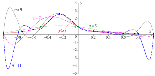
3.2.2. Using the Generalized Lagrange Interpolation

When the generalized Lagrange interpolation for an odd target function is applied, the condition that

y (0) = 0

is implicitly used. As a results, only five sampling points at

x

= 0.2, 0.4, 0.6, 0.8, 1.0 are used, and the corresponding Vandermonde matrix

V_{s}

and the vector

y_{s}

are

V_{s} = [\begin{matrix} 0.2 & 0.008 & 0.00032 & 1 \times 10^{- 5} & 5 \times 10^{- 7} \\ 0.4 & 0.064 & 0.01024 & 0.00164 & 0.00026 \\ 0.6 & 0.216 & 0.07776 & 0.02799 & 0.01008 \\ 0.8 & 0.512 & 0.32768 & 0.20972 & 0.13422 \\ 1.0 & 1.000 & 1.00000 & 1.00000 & 1.00000 \end{matrix}],

y_{s} = \{\begin{matrix} 0.19738 \\ 0.37995 \\ 0.53705 \\ 0.66404 \\ 0.76159 \end{matrix}\}, V_{s}^{- 1} y_{s} = \{\begin{matrix} 0.99999 \\ - 0.33311 \\ 0.13127 \\ - 0.04652 \\ 0.00997 \end{matrix}\} .

Using equation (22), the numerical derivatives are evaluated, and the results are presented in Table 8, in which the relative errors range from -0.045% to 0.0032%. From equation (24), the numerical integral is

I = \int_{0}^{1} \tanh (x) dx = \{\frac{1}{2} \frac{1}{4} \frac{1}{6} \frac{1}{8} \frac{1}{10}\} V_{s}^{- 1} y_{s} = 0.4337782661,

and the relative error is -0.0006%. These results demonstrate a clear advantage in accuracy of the generalized Lagrange interpolation over the classical Lagrange interpolation method.

Table 8. Numerical differentiation using the generalized Lagrange interpolation.

$x$	0.1	0.3	0.5	0.7	0.9
Exact values	0.99007	0.91514	0.78645	0.63474	0.48692
Numerical values	0. 99007	0. 91514	0.78644	0.63476	0.48670
Error (%)	0	0	$- 1.27 \times 10^{- 5}$	0.0032	-0.0452

3.3. Example 3 - Root of a Function

Consider the even function

y (x) = \cos x - x^{2}

. The exact root of

y (x)

within the interval [0, 1] is

x =

0.824132312, which serves as a reference for evaluating the efficiency and accuracy of the results obtained using the proposed method.

The Taylor series expansion of the function

y (x)

y (x) = \cos x - x^{2} = 1 - \frac{3}{2} x^{2} + \frac{1}{4!} x^{4} + ο (\frac{x^{6}}{6!}) .

It shows that if a three-point generalized Lagrange interpolation for even function is used, the square of the estimated root is governed by a quadratic equation, the root of which is readily calculated.

3.3.1. The First Iteration

Sample the function at three points with regular intervals as listed in Table 9.

Table 9. Sampling points for the first iteration.

$x$	0.75	0.875	1.0
$y$	0.169188869	-0.124628142	-0.459697694

By using these three sampling points and applying equation (16), the corresponding Vandermonde matrix

V_{s}

and the vector

y_{s}

are

V_{s} = [\begin{matrix} 1 & 0.562500 & 0.316406250 \\ 1 & 0.765625 & 0.586181641 \\ 1 & 1.000000 & 1.000000000 \end{matrix}],

y_{s} = \{\begin{matrix} 0.169188869 \\ - 0.124628142 \\ - 0.459697694 \end{matrix}\}, V_{s}^{- 1} y_{s} = \{\begin{matrix} 0.999426292 \\ - 1.497646627 \\ 0.038522640 \end{matrix}\} .

The root of the function

y (x)

is obtained by setting equation (15) equal to zero as follows:

y (x) = \{1 x^{2} x^{4}\} V_{s}^{- 1} y_{s} = 0.999426292 - 1.497646627 x^{2} + 0.03852264 x^{4} = 0,

from which the root in the interval [0, 1] is

x =

0.8241341. The relative error with respect to the exact root in the first iteration is 0.0002%.

3.3.2. The Second Iteration

To improve the accuracy, a new set of three sampling points is selected for this iteration as shown in Table 10. The root found in the first iteration is used as the centre point, and the interval of the sampling point can be reduced significantly as the root in the first iteration is already quite accurate.

Table 10. Sampling points for the second iteration.

$x$	0.814	0.824	0.834
$y$	0.023999776	0.000315174	-0.023637357

The corresponding Vandermonde matrix

V_{s}

and the vector

y_{s}

are given by

V_{s} = [\begin{matrix} 1 & 0.662596 & 0.439033459 \\ 1 & 0.678976 & 0.461008409 \\ 1 & 0.695556 & 0.483798149 \end{matrix}],

y_{s} = \{\begin{matrix} 0.023999776 \\ 0.000315174 \\ - 0.023637357 \end{matrix}\}, V_{s}^{- 1} y_{s} = \{\begin{matrix} 0.999581006 \\ - 1.498140511 \\ 0.038905190 \end{matrix}\} .

The root of the function

y (x)

is obtained by

y (x) = \{1 x^{2} x^{4}\} V_{s}^{- 1} y_{s} = 0.999581006 - 1.498140511 x^{2} + 0.038905190 x^{4} = 0,

from which the corresponding root is determined as

x =

0.824132312, which is the same as the exact root.

It is demonstrated that the proposed method can achieve a high-accuracy numerical solution with only two iterations. By employing this approach, one can avoid the shortcomings of

y^{'} = 0

and a non-convergent loop that may occur in the Newton-Raphson formula. Moreover, at any stage of the iteration, three new appropriate samples can be chosen to fit.

3.4. Example 4 - Extrema of a Function

Consider the odd function

y (x) = 10 \sin x - \tan x

. In the interval [0, 1.5], the maximum value

y_{\max} =

6.949224835 occurs at

x =

1.088111560.

3.4.1. The First Iteration

Sample the function at three points with regular intervals as listed in Table 11.

Table 11. Sampling points for the first iteration.

$x$	1.0	1.1	1.2
$y$	6.857302123	6.947313944	6.748239238

By using these three sampling points and applying equation (21), the corresponding Vandermonde matrix

V_{s}

and the vector

y_{s}

are

V_{s} = [\begin{matrix} 1.0 & 1.000 & 1.00000 \\ 1.1 & 1.331 & 1.61051 \\ 1.2 & 1.728 & 2.48832 \end{matrix}],

y_{s} = \{\begin{matrix} 6.857302123 \\ 6.947313944 \\ 6.748239238 \end{matrix}\}, V_{s}^{- 1} y_{s} = \{\begin{matrix} 8.251664187 \\ - 0.415431956 \\ - 0.978930108 \end{matrix}\} .

The critical point of function

y (x)

is obtained by setting

equation (22) equal to zero, as follows:

y^{'} (x) = \{1 {3 x}^{2} {5 x}^{4}\} V_{s}^{- 1} y_{s} = 8.251664187 - 1.246295867 x^{2} - 4.894650541 x^{4} = 0,

from which the root in the interval [0, 1.5] is

x =

1.085043282, and the corresponding extremum of

y (x)

is given by

y (1.085043282) = 10 \sin (1.085043282) - \tan (1.085043282) = 6.949100305 .

The relative error with respect to the exact extremum in the first iteration is −0.00179%.

3.4.2. The Second Iteration

To improve the accuracy, a new set of three sampling points is selected for this iteration as shown in Table 12. As in Example 3, the centre point is chosen as the root in the first iteration, and the interval of sampling is significantly reduced.

Table 12. Sampling points for the second iteration.

$x$	1.080	1.085	1.090
$y$	6.948360731	6.949096775	6.949177322

The corresponding Vandermonde matrix

V_{s}

and the vector

y_{s}

are given by

V_{s} = [\begin{matrix} 1.080 & 1.259712000 & 1.469328077 \\ 1.085 & 1.277289125 & 1.503656690 \\ 1.090 & 1.295029000 & 1.538623955 \end{matrix}],

y_{s} = \{\begin{matrix} 6.948360731 \\ 6.949096775 \\ 6.949177322 \end{matrix}\}, V_{s}^{- 1} y_{s} = \{\begin{matrix} 8.381084461 \\ - 0.672249549 \\ - 0.855064082 \end{matrix}\} .

The critical point of function

y (x)

is obtained by

y^{'} (x) = \{1 {3 x}^{2} {5 x}^{4}\} V_{s}^{- 1} y_{s} = 8.381084461 - 2.016748647 x^{2} - 4.275320409 x^{4} = 0,

from which the root is determined as

x =

1.088112745, and the corresponding local extremum of

y (x)

y (1.088112745) = 10 \sin (1.088112745) - \tan (1.088112745) = 6.949224834 .

which is the same as the exact extremum up to the eighth decimal place. Using equation (23), the value of the second-order derivative at the critical point is

y^{''} (1.088112745) = - 26.42 < 0,

indicating that the local extremum 6.949224834 is a maximum.

3.5. Example 5 - Functions Exhibiting Runge Phenomenon

As discussed in Section 1, when interpolating certain functions in a finite interval using the classical Lagrange interpolation, there may be large oscillations and divergence close to the endpoints of the interpolation intervals, resulting in the so-called Runge phenomenon.

The Runge phenomenon can be effectively eliminated by applied the generalized Lagrange interpolation with appropriate coordinate functions. Without loss of generality, consider a function

f (z)

with end points

(a, α)

and

(b, β)

. By adding a linear function

f (z)

y (z) = f (z) - \frac{βa - αb}{a - b} - \frac{α - β}{a - b} z,

(25)

the endpoints of function

y (z)

can be transformed to

(a, 0)

and

(b, 0)

. By a change of variable

z = a + (b - a) x

, the domain of function

y (x)

becomes [0, 1].

Because function

y (x)

satisfies the boundary conditions

y (0) = 0

and

y (1) = 0

, while

y^{'} (0) \neq 0

and

y^{'} (1) \neq 0

, the shape functions of the free vibration of a simply supported beam of length

L = 1

can be employed as the coordinate functions, which satisfy the required boundary conditions and are given by

φ_{n} (x) = \sin (nπx), n

=1, 2, ....(26)

To illustrate, consider the function in equation (4), or

f (z) = \frac{1}{1 + 5 z + 10 z^{2}}, - 1 \leq z \leq 1,

with endpoints (-1, 1/6) and (1, 1/16). Using equation (25), function

y (z) = \frac{1}{1 + 5 z + 10 z^{2}} - \frac{11}{96} + \frac{5}{96} z, - 1 \leq z \leq 1,

has endpoints (-1, 0) and (1, 0). Letting

z = - 1 + 2 x

, the transformed function

y (x) = \frac{1}{6 - 30 x + 40 x^{2}} - \frac{1}{6} + \frac{5}{48} x, 0 \leq x \leq 1,

(27)

has endpoints (0, 0) and (1, 0).

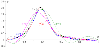
3.5.1. Classical Lagrange Interpolation

Sample the function

y (x)

in equation (25) using

n

equally spaced points within the interval

0 \leq x \leq 1 : x_{i} = \frac{i}{n - 1}, i

=0, 1, 2, ...,

n - 1

. For

n

=11, the corresponding Vandermonde matrix

V_{s}

and the vector

y_{s}

are given by

V_{s} = {[\begin{matrix} 1 & 0 & 0 & \dots & 0 \\ 1 & 0.1 & 0.01 & \dots & 1 \times 10^{- 10} \\ 1 & 0.2 & 0.04 & \dots & 1 \times 10^{- 7} \\ ⋮ & ⋮ & ⋮ & ⋱ & ⋮ \\ 1 & 1 & 1 & \dots & 1 \end{matrix}]}_{11 \times 11},

y_{s} = {\{\begin{matrix} 0 \\ 0.13787 \\ 0.47917 \\ ⋮ \\ 0 \end{matrix}\}}_{11 \times 1}, V_{s}^{- 1} y_{s} = {\{\begin{matrix} 0 \\ - 372.879 \\ 10182.083 \\ ⋮ \\ 4.543 \times 10^{5} \end{matrix}\}}_{11 \times 1} .

For equation (13), the expression for the classical Lagrange interpolation is

y (x) = \{\begin{matrix} 1 & x & x^{2} & \dots & x^{10} \end{matrix}\} V_{s}^{- 1} y_{s},

which is shown in Figure 2(a) as black dashed line. It is seen that the classical Lagrange interpolation exhibits the typical Runge phenomenon near the endpoints of the interval.

3.5.2. Generalized Lagrange Interpolation

The shape functions

φ_{n} (x)

in equation (26) are employed as coordinate functions. Because the conditions

y (0) = y (1) = 0

are inherently satisfied, nine sampling points at

x

=0.1, 0.2, 0.3, ..., 0.9 are used. The corresponding Vandermonde matrix

V_{s}

and the vector

y_{s}

are

V_{s} = {[\begin{matrix} 0.30902 & 0.58779 & 0.80902 & \dots & 0.30902 \\ 0.58779 & 0.95106 & 0.95106 & \dots & - 0.58779 \\ 0.80902 & 0.95106 & 0.30902 & \dots & 0.80902 \\ ⋮ & ⋮ & ⋮ & ⋱ & ⋮ \\ 0.30902 & - 0.58779 & 0.80902 & \dots & 0.30902 \end{matrix}]}_{9 \times 9}

y_{s} = {\{\begin{matrix} 0.13787 \\ 0.47917 \\ 1.53125 \\ ⋮ \\ 0.01480 \end{matrix}\}}_{9 \times 1}, V_{s}^{- 1} y_{s} = {\{\begin{matrix} 0.00849 \\ 0.01364 \\ 0.01142 \\ ⋮ \\ 0.00024 \end{matrix}\}}_{9 \times 1} .

Using equation (8), the expression for the generalized Lagrange interpolation is

y (x) = \{\begin{matrix} \sin (πx) & \sin (2 πx) & \dots & \sin (9 πx) \end{matrix}\} V_{s}^{- 1} y_{s},

which is shown in Figure 2(b) as blue dashed line.

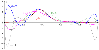
(a). Classical Lagrange interpolation. (b). Generalized Lagrange interpolation.

Download: Download full-size image

Figure 2. Comparison between numerical and exact results.

It is observed that the generalized Lagrange interpolation method effectively eliminates the Runge phenomenon and demonstrates significantly higher approximation accuracy across the entire domain as compared to the classical Lagrange interpolation. As the number of sampling points increases, the Runge phenomenon in the classical method becomes more pronounced, whereas the accuracy of the generalized Lagrange interpolation is further improved.

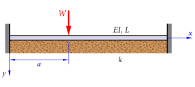
3.6. Example 6 - Deformation of a Beam on Elastic Foundation

Consider a beam AB on elastic foundation, which is clamped at both ends, as shown in Figure 3. The beam is subjected to a concentrated load

L

, the width of the beam is

b

, the moment of inertia is

I

, and the Young’s modulus is

E

. From Winkler’s assumption,

k = k_{0} b

, where

k_{0}

is the modulus of the foundation.

Download: Download full-size image

Figure 3. Clamped-clamped beam on elastic foundation.

By using Dirac delta function, the concentrated load can be expressed as

w (x) = Wδ (x - a) .

The differential equation governing the deflection

y (x)

[23]

\frac{d^{4} y (x)}{d x^{4}} + 4 β^{4} y (x) = \hat{W} δ (x - a),

(28)

4 β^{4} = \frac{k}{EI}, \hat{W} = \frac{W}{EI} .

Because both ends of the beam are clamped, the boundary conditions are

y (0) = y (L) = y^{'} (0) = y^{'} (L) = 0 .

Applying the method of Laplace transform, it can be shown that the solution of differential equation (28) is

y (x) = y^{''} (0) ϕ_{1} (x) + y^{'''} (0) ϕ_{0} (x) + \hat{W} ϕ_{0} (x - a) H (x - a)

(29)

in which

ϕ_{0} (x) = \frac{1}{4 β^{3}} (\sin βx \cosh βx - \cos βx \sinh βx),

ϕ_{1} (x) = \frac{1}{2 β^{2}} \sin βx \sinh βx,

ϕ_{2} (x) = \frac{1}{2 β} (\sin βx \cosh βx + \cos βx \sinh βx) .

From the boundary conditions

y (L) = y^{'} (L) = 0,

y'' (0)

and

y''' (0)

can be determined as

y^{''} (0) = \frac{α_{0} ϕ_{1} (L) - α_{1} ϕ_{0} (L)}{ϕ_{1}^{2} (L) - ϕ_{0} (L) ϕ_{2} (L)},

y^{'''} (0) = \frac{α_{1} ϕ_{1} (L) - α_{0} ϕ_{2} (L)}{ϕ_{1}^{2} (L) - ϕ_{0} (L) ϕ_{2} (L)},

where

α_{0} = - \hat{W} ϕ_{0} (L - a), α_{1} = - \hat{W} ϕ_{1} (L - a) .

In order to induce significant deflection in the beam for illustrative purposes, the following parameters are adopted: Young’s modulus

E

=100Gpa, the width, thickness, and height of the beam are

b

=1m,

h

=3m,

L

=20m, the modulus of the foundation

k_{0} =1.125× 10^{11}

N/m³, and the concentrated load

W

=22.5 GN. Thus,

\hat{W} = W / EI

= 0.1 and

β = {(k / 4 EI)}^{1 / 4}

=0.5946, in which the moment of inertia is calculated as

I = b h^{3} / 12

3.6.1. Numerical Beam Deflection by the Classical Lagrange Interpolation

Eleven sample points are selected at

x

=0, 2, 4, 6, ..., 20. From the analytical deflection (29), the corresponding Vandermonde matrix

V_{s}

and the vector

y_{s}

are given by

V_{s} = {[\begin{matrix} 1 & 0 & 0 & \dots & 0 \\ 1 & 2 & 4 & \dots & 1024 \\ 1 & 4 & 16 & \dots & 1048576 \\ ⋮ & ⋮ & ⋮ & ⋱ & ⋮ \\ 1 & 20 & 400 & \dots & 1.024 \times 10^{13} \end{matrix}]}_{11 \times 11},

y_{s} = {\{\begin{matrix} 0 \\ 0.00835 \\ 0.04548 \\ ⋮ \\ 4 {\times 10}^{- 7} \end{matrix}\}}_{11 \times 1}, V_{s}^{- 1} y_{s} = {\{\begin{matrix} 0 \\ 0.19791 \\ - 0.27483 \\ ⋮ \\ - 4 {\times 10}^{- 10} \end{matrix}\}}_{11 \times 1} .

According to equation (13), the expression for the beam deflection from Lagrange interpolation is

y (x) = \{\begin{matrix} 1 & x & x^{2} & \dots & x^{10} \end{matrix}\} V_{s}^{- 1} y_{s},

which is shown in Figure 5 as black dashed line.

3.6.2. Numerical Beam Deflection by the Generalized Lagrange Interpolation

The shape functions of a supported beam are usually derived from the eigen-solutions of its free vibration. If the boundary characteristics of a supported beam, such as end displacements and rotations, are consistent with those of a more complex structural element, the shape functions of the beam can be employed as coordinate functions, so that the boundary conditions are satisfied intrinsically.

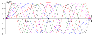
For a beam of length

L

with clamped-clamped boundary conditions, the

n

modal shape function of free vibration is given by

φ_{n} (ξ) = \cos h (λ_{n} ξ) - \cos (λ_{n} ξ)

- \frac{\cos h λ_{n} - \cos λ_{n}}{\sin h λ_{n} - \sin λ_{n}} [\sin h (λ_{n} ξ) - \sin (λ_{n} ξ)],

(30)

where

ξ = x / L

, and

λ_{n}

denotes the n th positive root of the characteristic equation

\cosh λ \cos λ = 1 .

The characteristic roots of the first nine modes are listed in Table 13, and the corresponding beam shape-functions are shown in Figure 4.

Table 13. Values of

λ

$n$	1	2	3	4	5
$λ_{n}$	4.7300	7.8532	10.9956	14.1372	17.2788
$n$	6	7	8	9
$λ_{n}$	20.4204	23.5619	26.7035	29.8451

Download: Download full-size image

Figure 4. Shape functions of the first nine beam modes.

Selecting nine sampling points at

x

=2, 4, 6, 8, ..., 18 m, the corresponding Vandermonde matrix

V_{s}

and the vector

y_{s}

are

V_{s} = {[\begin{matrix} 0.18910 & 0.45574 & 0.77005 & \dots & 1.19469 \\ 0.61939 & 1.20675 & 1.50783 & \dots & - 1.25752 \\ 1.09600 & 1.50550 & 0.86863 & \dots & 1.34513 \\ ⋮ & ⋮ & ⋮ & ⋱ & ⋮ \\ 0.18910 & - 0.45574 & 0.77005 & \dots & 0.98769 \end{matrix}]}_{9 \times 9},

y_{s} = {\{\begin{matrix} 0.00835 \\ 0.04548 \\ 0.04548 \\ ⋮ \\ 2.7 {\times 10}^{- 5} \end{matrix}\}}_{9 \times 1}, V_{s}^{- 1} y_{s} = {\{\begin{matrix} 0.00849 \\ 0.01364 \\ 0.01142 \\ ⋮ \\ 0.00024 \end{matrix}\}}_{9 \times 1} .

By applying equation (8), the deflection

y (x)

obtained using the generalized Lagrange interpolation is given by

y (x) = \{φ_{1} (x) φ_{2} (x) φ_{3} (x) \dots φ_{9} (x)\} V_{s}^{- 1} y_{s},

which is shown in Figure 5 as blue dashed line.

Download: Download full-size image

Figure 5. Comparison between numerical and exact results.

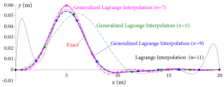
Figure 5 presents a comparison of beam deflections obtained using the classical Lagrange interpolation, the generalized Lagrange interpolation, and the exact theoretical solution. It can be observed that the classical Lagrange interpolation yields accurate results only near the mid-span of the beam. Close to the boundaries, the accuracy of the interpolation result deteriorates rapidly, leading to the Runge phenomenon with significant discrepancies from the exact solution.

In contrast, the generalized Lagrange interpolation demonstrates high accuracy across the entire beam, even with fewer sampling points. More accurate solutions are achieved for

n \geq

7, with fitting performance further improving as

n

increases. This is attributed to the fact that the boundary conditions are inherently embedded in the coordinate functions, which markedly enhances convergence near the boundaries and effectively eliminates the Runge phenomenon commonly observed with classical Lagrange polynomials.

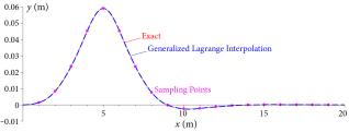
The result of generalized Lagrange interpolation, when nineteen sampling points at

x

=1, 2, ..., 19 (m) are used, is shown in Figure 6. It is seen that the result agrees with the exact result extremely well, with almost no visual difference.

It is noted that, for the classical Lagrange interpolation, two extra sampling points at

x

=0, 20 (m) are needed, and the Runge phenomenon is very severe, especially at the left end. The overall performance of the classical Lagrange interpolation does not improve by using more sampling points due to the Runge phenomenon.

(a) (b)

4. Discussions and Conclusions

It is evident that the classical Lagrange interpolation performs comparably to Stirling's stencil for first derivatives, matches the central difference scheme for second derivatives, and outperforms Simpson's rule for definite integration. However, its performance deteriorates when applied to symmetric or antisymmetric target functions, and it becomes invalid when boundary conditions are imposed. Moreover, the classical Lagrange interpolation exhibits a strong Runge phenomenon in the application of Runge-type functions.

In this study, a generalized Lagrange interpolation formula is proposed to improve the classical Lagrange interpolation, effectively overcoming the commonly observed Runge phenomenon, and thereby extending its range of applicability. The general n-point formulation of the proposed method is presented in equation (8).

According to the type of the target function, the generalized Lagrange interpolation formula selects appropriate coordinate functions to ensure that the interpolation inherently possesses key properties of the target function. Specifically, for asymmetric, symmetric, and antisymmetric target functions, consecutive-power, even-power, and odd-power polynomials are employed, respectively. For Runge-type functions or functions with prescribed boundary conditions, admissible shape functions are adopted as coordinate functions.

To illustrate the approach, six representative examples are presented: an even function, an odd function, root-finding of an even function, determining extrema of an odd function, a function exhibiting severe Runge phenomenon, and the deflection of a loaded beam on elastic foundation subject to prescribed boundary conditions. The use of appropriate coordinate functions improves convergence and enhances the overall accuracy of the numerical results.

Validation through numerical examples confirms that the proposed method effectively eliminates the Runge phenomenon and consistently outperforms the classical Lagrange interpolation in numerical differentiation, numerical integration, root-finding, and determining extrema tasks, demonstrating its versatility in handling symmetric and antisymmetric target functions. When applied to Runge-type functions, the generalized approach yields higher accuracy and better numerical stability, particularly in regions near the boundaries where the classical interpolation tends to diverge. Notably, the generalized Lagrange interpolation maintains high levels of accuracy, efficiency, and stability, all of which are further enhanced as the number of sampling points increases.

To ensure numerical accuracy and stability in practical applications of generalized Lagrange interpolation, the following guidelines are recommended:

When sampling points are evenly spaced, appropriate coordinate functions should be selected based on the properties of the target function to avoid the Runge phenomenon.

The magnitudes of sample values are to be comparable, and large discrepancies in scale should be avoided.

Using an appropriate transformation, the domain and boundary conditions can be modified as illustrated in Example 5, so that well-known coordinate functions can be applied to achieve more accurate and stable results.

The existing methodologies to resolve Runge's phenomenon primarily rely on the use of Chebyshev nodes or spline interpolation. In contrast, the proposed generalized Lagrange interpolation that uses collocation to determine the coefficients of expansion, similar to Galerkin's method of least square residues, offers a more robust, versatile, and simple alternative by employing admissible shape functions as coordinate functions. Whether applied to numerical differentiation, numerical definite integration, root-finding, determining extrema, or the solution of ordinary differential equations with imposed boundary conditions, this method consistently achieves high levels of accuracy, stability, and numerical efficiency.

Funding

This work is not supported by any external funding.

Data Availability Statement

The data is available from the corresponding author upon reasonable request.

Conflicts of Interest

The authors declare no conflicts of interest.

References

[1]	Liszka T. An interpolation method for an irregular net of nodes, International Journal for Numerical Methods in Engineering. 1984, 20(9): 1599-1612. https://doi.org/10.1002/nme.1620200905
[2]	Curtiss J. Interpolation in regularly distributed points, Transactions of the American Mathematical Society. 1935, 38(3): 458-473. https://doi.org/10.2307/1989807
[3]	Blu T, Thévenaz P, Unser M. Linear interpolation revitalized, IEEE Transactions on Image Processing. 2004, 13(5): 710-719. https://doi.org/10.1109/TIP.2004.826093
[4]	Greville T N E. Numerical procedures for interpolation by spline functions, Journal of the Society for Industrial and Applied Mathematics. Series B: Numerical Analysis, 1964, 1(1): 53-68.
[5]	Wang, R, Ly, B, Xie, W, Pandey, M. Lagrange Interpolation in Matrix Form for Numerical Differentiation and Integration, American Journal of Applied Mathematics. 2024, 12(3), 66-78. https://doi.org/10.11648/j.ajam.20241203.13
[6]	Runge C. Über empirische Funktionen und die Interpolation zwischen äquidistanten Ordinaten, Zeitschrift für Mathematik und Physik. 1901, 46(224-243): 20.
[7]	Boyd J P. Trouble with Gegenbauer reconstruction for defeating Gibbs’ phenomenon: Runge phenomenon in the diagonal limit of Gegenbauer polynomial approximations, Journal of Computational Physics. 2005, 204(1): 253-264. https://doi.org/10.1016/j.jcp.2004.10.008
[8]	Chen Y J, He H Y, Zhang S L. A new algebra interpolation polynomial without Runge phenomenon, Applied Mechanics and Materials. 2013, 303: 1085-1088. https://doi.org/10.4028/www.scientific.net/AMM.303-306.1085
[9]	Piret C. A radial basis function based frames strategy for bypassing the Runge phenomenon [J]. SIAM Journal on Scientific Computing, 2016, 38(4): A2262-A2282. https://doi.org/10.1137/15M1040943
[10]	Majidian H. Creating stable quadrature rules with preassigned points by interpolation, Calcolo. 2016, 53(2): 217-226. https://doi.org/10.1007/s10092-015-0145-0
[11]	She J, Tan Y. Research on Runge phenomenon, Computational and Mathematical Biophysics. 2019, 8(8): 1500-1510. https://doi.org/10.12677/AAM.2019.88175
[12]	Zhang R J, Liu X. Rational interpolation operator with finite Lebesgue constant, Calcolo. 2022, 59(1): 10. https://doi.org/10.1007/s10092-021-00454-1
[13]	Boyd J P. Defeating the Runge phenomenon for equispaced polynomial interpolation via Tikhonov regularization, Applied mathematics letters. 1992, 5(6): 57-59. https://doi.org/10.1016/0893-9659(92)90014-Z
[14]	Gottlieb D, Shu C W. Resolution properties of the Fourier method for discontinuous waves, Computer methods in applied mechanics and engineering. 1994, 116(1-4): 27-37. https://doi.org/10.1016/S0045-7825(94)80005-7
[15]	Boyd J P. A comparison of numerical algorithms for Fourier extension of the first, second, and third kinds, Journal of Computational Physics. 2002, 178(1): 118-160. https://doi.org/10.1006/jcph.2002.7023
[16]	Gelb A. Parameter optimization and reduction of round off error for the Gegenbauer reconstruction method, Journal of Scientific Computing. 2004, 20(3): 433-459. https://doi.org/10.1023/B:JOMP.0000025933.39334.17
[17]	Jackiewicz Z. Determination of Optimal Parameters for the Chebyshev--Gegenbauer Reconstruction Method, SIAM Journal on Scientific Computing. 2004, 25(4): 1187-1198. https://doi.org/10.1137/S1064827503423597
[18]	Jung J H, Shizgal B D. Generalization of the inverse polynomial reconstruction method in the resolution of the Gibbs phenomenon, Journal of computational and applied mathematics. 2004, 172(1): 131-151. https://doi.org/10.1016/j.cam.2004.02.003
[19]	Platte R B, Driscoll T A. Polynomials and potential theory for Gaussian radial basis function interpolation, SIAM Journal on Numerical Analysis. 2005, 43(2): 750-766. https://doi.org/10.1137/040610143
[20]	Boyd J P, Ong J R. Exponentially-convergent strategies for defeating the Runge phenomenon for the approximation of non-periodic functions, part I: single-interval schemes, Comput. Phys. 2009, 5(2-4): 484-497.
[21]	Lin H, Sun L. Searching globally optimal parameter sequence for defeating Runge phenomenon by immunity genetic algorithm, Applied Mathematics and Computation. 2015, 264: 85-98. https://doi.org/10.1016/j.amc.2015.04.069
[22]	Blevins R D, Plunkett R. Formulas for natural frequency and mode shape, Journal of Applied Mechanics. 1980, 47(2): 461. https://doi.org/10.1115/1.3153712
[23]	Xie W C. Differential equations for engineers. Cambridge university press, 2010.

Cite This Article

Plain Text BibTeX RIS

APA Style

Cheng, Z., Xie, W., Pandey, M., Ly, B. (2026). Versatility of the Generalized Lagrange Interpolation Formula in the Matrix Form. American Journal of Applied Mathematics, 14(1), 14-26. https://doi.org/10.11648/j.ajam.20261401.13

Copy | Download

ACS Style

Cheng, Z.; Xie, W.; Pandey, M.; Ly, B. Versatility of the Generalized Lagrange Interpolation Formula in the Matrix Form. Am. J. Appl. Math. 2026, 14(1), 14-26. doi: 10.11648/j.ajam.20261401.13

Copy | Download

AMA Style

Cheng Z, Xie W, Pandey M, Ly B. Versatility of the Generalized Lagrange Interpolation Formula in the Matrix Form. Am J Appl Math. 2026;14(1):14-26. doi: 10.11648/j.ajam.20261401.13

Copy | Download

@article{10.11648/j.ajam.20261401.13,
  author = {Zhengquan Cheng and Wei-Chau Xie and Mahesh Pandey and Binh-Le Ly},
  title = {Versatility of the Generalized Lagrange Interpolation Formula in the Matrix Form},
  journal = {American Journal of Applied Mathematics},
  volume = {14},
  number = {1},
  pages = {14-26},
  doi = {10.11648/j.ajam.20261401.13},
  url = {https://doi.org/10.11648/j.ajam.20261401.13},
  eprint = {https://article.sciencepublishinggroup.com/pdf/10.11648.j.ajam.20261401.13},
  abstract = {In this paper, a generalized Lagrange interpolation formula expressed in matrix form is developed to systematically expand a sampled function with enhanced flexibility and computational rigor. The proposed formulation employs appropriate coordinate functions that not only satisfy prescribed boundary conditions but also exploit the symmetry or anti-symmetry inherent in the function under consideration. When such conditions are absent, the coordinate functions naturally degenerate into polynomial bases, thereby reproducing the classical Lagrange interpolation as a special case. The expansion coefficients are efficiently obtained through the collocation method, ensuring numerical simplicity and stability. The matrix-based generalized Lagrange interpolation exhibits substantial versatility beyond traditional interpolation tasks. It can be readily applied to numerical differentiation and integration under both uniform and non-uniform sampling schemes. Moreover, the approach proves useful in solving ordinary differential equations with specified boundary constraints, as well as in problems involving root-finding and extremum detection of functions. Numerical experiments demonstrate the accuracy and robustness of the proposed method, revealing a marked reduction in the Runge phenomenon even when the number of sampling points is limited. The results further indicate that computational efficiency and precision improve progressively as the number of samples increases. Overall, the generalized interpolation framework developed herein provides a unified and reliable computational tool for interpolation, differentiation, integration, and boundary-value problems, thereby offering broad potential for applications in numerical analysis and scientific computing.},
 year = {2026}
}

Copy | Download

TY  - JOUR
T1  - Versatility of the Generalized Lagrange Interpolation Formula in the Matrix Form
AU  - Zhengquan Cheng
AU  - Wei-Chau Xie
AU  - Mahesh Pandey
AU  - Binh-Le Ly
Y1  - 2026/01/20
PY  - 2026
N1  - https://doi.org/10.11648/j.ajam.20261401.13
DO  - 10.11648/j.ajam.20261401.13
T2  - American Journal of Applied Mathematics
JF  - American Journal of Applied Mathematics
JO  - American Journal of Applied Mathematics
SP  - 14
EP  - 26
PB  - Science Publishing Group
SN  - 2330-006X
UR  - https://doi.org/10.11648/j.ajam.20261401.13
AB  - In this paper, a generalized Lagrange interpolation formula expressed in matrix form is developed to systematically expand a sampled function with enhanced flexibility and computational rigor. The proposed formulation employs appropriate coordinate functions that not only satisfy prescribed boundary conditions but also exploit the symmetry or anti-symmetry inherent in the function under consideration. When such conditions are absent, the coordinate functions naturally degenerate into polynomial bases, thereby reproducing the classical Lagrange interpolation as a special case. The expansion coefficients are efficiently obtained through the collocation method, ensuring numerical simplicity and stability. The matrix-based generalized Lagrange interpolation exhibits substantial versatility beyond traditional interpolation tasks. It can be readily applied to numerical differentiation and integration under both uniform and non-uniform sampling schemes. Moreover, the approach proves useful in solving ordinary differential equations with specified boundary constraints, as well as in problems involving root-finding and extremum detection of functions. Numerical experiments demonstrate the accuracy and robustness of the proposed method, revealing a marked reduction in the Runge phenomenon even when the number of sampling points is limited. The results further indicate that computational efficiency and precision improve progressively as the number of samples increases. Overall, the generalized interpolation framework developed herein provides a unified and reliable computational tool for interpolation, differentiation, integration, and boundary-value problems, thereby offering broad potential for applications in numerical analysis and scientific computing.
VL  - 14
IS  - 1
ER  -

Copy | Download

Author Information

Zhengquan Cheng

Department of Civil and Environmental Engineering, University of Waterloo, Ontario, Canada

Biography: Zhengquan Cheng is a PhD student in the Civil and Environmental Engineering department at the University of Waterloo.

Contact Email

http://orcid.org/0009-0009-3560-1344
Wei-Chau Xie

Department of Civil and Environmental Engineering, University of Waterloo, Ontario, Canada

Biography: Wei-Chau Xie is a Professor in the Civil and Environmental Engineering department at the University of Waterloo.

Contact Email

http://orcid.org/0000-0002-9761-7968
Mahesh Pandey

Department of Civil and Environmental Engineering, University of Waterloo, Ontario, Canada

Biography: Mahesh Pandey is a Professor in the Civil and Environmental Engineering department at the University of Waterloo.

Contact Email

http://orcid.org/0000-0002-5083-2599
Binh-Le Ly

Atomic Energy of Canada, Mississauga, Canada

Biography: Binh-Le Ly received PhD degree in University of Waterloo, and he worked at Atomic Energy of Canada.

Contact Email

Download PDF

Submit an Article

Plain Text BibTeX RIS

APA Style

Cheng, Z., Xie, W., Pandey, M., Ly, B. (2026). Versatility of the Generalized Lagrange Interpolation Formula in the Matrix Form. American Journal of Applied Mathematics, 14(1), 14-26. https://doi.org/10.11648/j.ajam.20261401.13

Copy | Download

ACS Style

Cheng, Z.; Xie, W.; Pandey, M.; Ly, B. Versatility of the Generalized Lagrange Interpolation Formula in the Matrix Form. Am. J. Appl. Math. 2026, 14(1), 14-26. doi: 10.11648/j.ajam.20261401.13

Copy | Download

AMA Style

Cheng Z, Xie W, Pandey M, Ly B. Versatility of the Generalized Lagrange Interpolation Formula in the Matrix Form. Am J Appl Math. 2026;14(1):14-26. doi: 10.11648/j.ajam.20261401.13

Copy | Download

@article{10.11648/j.ajam.20261401.13,
  author = {Zhengquan Cheng and Wei-Chau Xie and Mahesh Pandey and Binh-Le Ly},
  title = {Versatility of the Generalized Lagrange Interpolation Formula in the Matrix Form},
  journal = {American Journal of Applied Mathematics},
  volume = {14},
  number = {1},
  pages = {14-26},
  doi = {10.11648/j.ajam.20261401.13},
  url = {https://doi.org/10.11648/j.ajam.20261401.13},
  eprint = {https://article.sciencepublishinggroup.com/pdf/10.11648.j.ajam.20261401.13},
  abstract = {In this paper, a generalized Lagrange interpolation formula expressed in matrix form is developed to systematically expand a sampled function with enhanced flexibility and computational rigor. The proposed formulation employs appropriate coordinate functions that not only satisfy prescribed boundary conditions but also exploit the symmetry or anti-symmetry inherent in the function under consideration. When such conditions are absent, the coordinate functions naturally degenerate into polynomial bases, thereby reproducing the classical Lagrange interpolation as a special case. The expansion coefficients are efficiently obtained through the collocation method, ensuring numerical simplicity and stability. The matrix-based generalized Lagrange interpolation exhibits substantial versatility beyond traditional interpolation tasks. It can be readily applied to numerical differentiation and integration under both uniform and non-uniform sampling schemes. Moreover, the approach proves useful in solving ordinary differential equations with specified boundary constraints, as well as in problems involving root-finding and extremum detection of functions. Numerical experiments demonstrate the accuracy and robustness of the proposed method, revealing a marked reduction in the Runge phenomenon even when the number of sampling points is limited. The results further indicate that computational efficiency and precision improve progressively as the number of samples increases. Overall, the generalized interpolation framework developed herein provides a unified and reliable computational tool for interpolation, differentiation, integration, and boundary-value problems, thereby offering broad potential for applications in numerical analysis and scientific computing.},
 year = {2026}
}

Copy | Download

TY  - JOUR
T1  - Versatility of the Generalized Lagrange Interpolation Formula in the Matrix Form
AU  - Zhengquan Cheng
AU  - Wei-Chau Xie
AU  - Mahesh Pandey
AU  - Binh-Le Ly
Y1  - 2026/01/20
PY  - 2026
N1  - https://doi.org/10.11648/j.ajam.20261401.13
DO  - 10.11648/j.ajam.20261401.13
T2  - American Journal of Applied Mathematics
JF  - American Journal of Applied Mathematics
JO  - American Journal of Applied Mathematics
SP  - 14
EP  - 26
PB  - Science Publishing Group
SN  - 2330-006X
UR  - https://doi.org/10.11648/j.ajam.20261401.13
AB  - In this paper, a generalized Lagrange interpolation formula expressed in matrix form is developed to systematically expand a sampled function with enhanced flexibility and computational rigor. The proposed formulation employs appropriate coordinate functions that not only satisfy prescribed boundary conditions but also exploit the symmetry or anti-symmetry inherent in the function under consideration. When such conditions are absent, the coordinate functions naturally degenerate into polynomial bases, thereby reproducing the classical Lagrange interpolation as a special case. The expansion coefficients are efficiently obtained through the collocation method, ensuring numerical simplicity and stability. The matrix-based generalized Lagrange interpolation exhibits substantial versatility beyond traditional interpolation tasks. It can be readily applied to numerical differentiation and integration under both uniform and non-uniform sampling schemes. Moreover, the approach proves useful in solving ordinary differential equations with specified boundary constraints, as well as in problems involving root-finding and extremum detection of functions. Numerical experiments demonstrate the accuracy and robustness of the proposed method, revealing a marked reduction in the Runge phenomenon even when the number of sampling points is limited. The results further indicate that computational efficiency and precision improve progressively as the number of samples increases. Overall, the generalized interpolation framework developed herein provides a unified and reliable computational tool for interpolation, differentiation, integration, and boundary-value problems, thereby offering broad potential for applications in numerical analysis and scientific computing.
VL  - 14
IS  - 1
ER  -

Copy | Download