Robust Power System Optimization Using LSTM-Based Load Forecasting and AIS Algorithm

Randriamora Edmond; Rasolofonirina Tokiniaina Francky; Andriatsihoarana Harlin Samuel; Randriamaroson Rivo Mahandrisoa

doi:doi:10.11648/j.jeee.20261403.14

Research Article |

Robust Power System Optimization Using LSTM-Based Load Forecasting and AIS Algorithm

Randriamora Edmond^*, Rasolofonirina Tokiniaina Francky, Andriatsihoarana Harlin Samuel, Randriamaroson Rivo Mahandrisoa

Published in Journal of Electrical and Electronic Engineering (Volume 14, Issue 3)

Received: 3 April 2026 Accepted: 16 April 2026 Published: 16 May 2026

Views: Downloads:

Download PDF

Share This Article

Twitter
Linked In
Facebook

Abstract

Optimizing alternating current (AC) power flow under uncertainty remains a major challenge in modern power systems, particularly with the increasing penetration of variable renewable energy sources. This paper proposes a hybrid two-stage framework that integrates long short-term memory (LSTM) networks for load forecasting with an artificial immune system (AIS)-based optimization approach, embedded within a Monte Carlo simulation scheme to explicitly account for uncertainty. The methodology is validated on the IEEE 30-bus test system. In the first stage, the LSTM model captures temporal dependencies to generate short-term load forecasts, while in the second stage, these forecasts are incorporated into an AIS-based AC optimal power flow (AC-OPF) formulation. Monte Carlo simulations are employed to model stochastic variations and assess system performance across multiple scenarios. The results show that, although the reduction in operational cost is relatively marginal compared to deterministic approaches, the proposed framework significantly enhances the robustness and stability of OPF solutions under forecasting uncertainty, improving the system’s ability to maintain feasible and consistent operating points despite variability in load predictions. However, the forecasting performance of the LSTM model is sensitive to noise and out-of-distribution inputs, which may affect the overall optimization quality. Overall, the main contribution of this work lies in the development of an integrated forecasting–optimization framework that strengthens the reliability and resilience of power system operation under uncertainty.

Published in	Journal of Electrical and Electronic Engineering (Volume 14, Issue 3)
DOI	10.11648/j.jeee.20261403.14
Page(s)	152-162
Creative Commons	This is an Open Access article, distributed under the terms of the Creative Commons Attribution 4.0 International License (http://creativecommons.org/licenses/by/4.0/), which permits unrestricted use, distribution and reproduction in any medium or format, provided the original work is properly cited.
Copyright	Copyright © The Author(s), 2026. Published by Science Publishing Group

Keywords

AC Optimal Power Flow, LSTM, Artificial Immune System, Load Forecasting, Uncertainty, Monte Carlo Simulation, Robust Optimization

1. Introduction

The transition to smart and sustainable power grids has dramatically increased the complexity of managing modern power systems

[54, 55]

. The large-scale integration of uncontrollable renewable energy resources, such as wind and solar power, has introduced unprecedented spatial and temporal variability

[1]

. Unlike traditional grids based on predictable fossil fuel generators, contemporary grids must contend with dual uncertainties: the intermittency of generation on the supply side and the stochastic volatility of the load on the demand side

[9, 10]

. This dynamic requires sophisticated decision-making tools capable of ensuring grid stability while minimizing operational costs in an increasingly uncertain environment

[11, 12]

The classic optimal power flow problem aims to determine the most economical operating point of the grid under strict physical constraints

[56, 57]

. However, traditional deterministic OPF is insufficient in the face of modern uncertainties, as it does not guarantee the feasibility of solutions when actual parameters deviate from forecasts

[13]

. Therefore, robust optimization is necessary to ensure that the system remains within its operational limits, even under worst-case scenarios

[14]

. In this context, the accuracy of load forecasting is the cornerstone of planning; however, even a minor forecasting error can lead to violations of critical constraints or significant economic suboptimality during the subsequent optimization stage

[8, 15]

To address these challenges, the academic literature has adopted hybrid approaches. For short-term load forecasting, deep learning models, particularly long short-term memory (LSTM) networks, have become the standard owing to their ability to capture complex temporal dependencies and nonlinear trends in time series data

[2, 16]

. In parallel, to solve non-convex and non-smooth OPF problems (including valve point effects), metaheuristics such as genetic algorithms and particle swarm optimization have been widely used

[17, 18]

. Among these, the Artificial Immune System stands out for its robustness and global search capability, using clonal selection and hypermutation mechanisms to avoid local optima, often outperforming classical methods in rugged search landscapes

[3, 19]

Despite these advances, a methodological gap persists. Most current research treats LSTM-based forecasting and metaheuristic-based optimization as two isolated steps, thereby ignoring the dynamic interactions between the forecasting error and optimization feasibility

[8, 20]

. Very few studies have simultaneously integrated the LSTM predictive framework with the search power of AIS for AC-OPF while systematically quantifying robustness via Monte Carlo simulations

[21, 22]

. Furthermore, the vulnerability of LSTM models to noise and out-of-range input variables remains a critical limitation that has been little explored in the context of robust power flow optimization

[4, 5]

To address these gaps, this study makes the following contributions.

1) A hybrid LSTM-AIS framework is proposed to unify long-term temporal load forecasting with immunological metaheuristic search for enhanced grid dispatch efficiency.

2) A robust AC-OPF formulation under uncertainty is developed, explicitly considering non-linear constraints and valve-point loading effects often neglected in simplified models.

3) Monte Carlo scenarios are integrated to assess the statistical reliability of the optimal solutions and quantify the impact of forecast errors on system security.

4) Performance is validated on the IEEE 30-bus system, demonstrating significant reductions in operational costs and improved constraint satisfaction compared to traditional stochastic approaches.

2. Literature Review

The integration of load forecasting and power flow optimization under uncertainty is a rapidly expanding field driven by the need to manage increasingly complex and intermittent power grids. This review examines the state of the art between 2018 and 2025 in four critical areas.

2.1. Load Forecasting: LSTM vs. ARIMA vs. ANN

The accuracy of electricity demand forecasting is the first line of defence against grid instability. Traditional methods, such as ARIMA, have long been favored for their statistical simplicity

[23]

. However, recent comparative studies have demonstrated that ARIMA struggles to capture complex nonlinear relationships and generates high forecasting errors, particularly over 24-hour horizons

[24]

. ANNs have brought significant improvements by handling nonlinearity; however, they often suffer from the vanishing gradient problem and an inability to model long-term temporal dependencies

[25]

LSTM, a variant of recurrent neural networks, has established itself as the go-to solution between 2020 and 2024

[26, 27]

. Unlike traditional ANNs, LSTM uses “gate” mechanisms to retain or discard information over long periods, which is crucial for cyclic load profiles

[23]

. Nevertheless, a major criticism of LSTM lies in its sensitivity to noise and its tendency to overfit when input data deviate from the training conditions, which can compromise the reliability of downstream optimization decisions

[5]

2.2. OPF Optimization: Classical vs. Metaheuristics

The OPF problem is inherently non-convex and nonlinear, especially when it incorporates effects such as valve-point loading

[28, 29, 52]

. Classical computational methods, such as quadratic programming or the interior-point method, offer fast convergence and algebraic efficiency for smooth problems

[28, 30]

. However, they are often criticized for their tendency to become stuck in local optima and their inability to handle non-differentiable objective functions

[28, 31]

To overcome these limitations, metaheuristics have been developed. Particle Swarm Optimization (PSO) and Genetic Algorithms (GA) are widely used for their ability to perform global searches

[32, 33]

. Recent studies (2022–2024) suggest that metaheuristic approaches can outperform traditional convex optimization in terms of solution quality for complex distribution systems, despite their higher computational costs and sensitivity to parameter tuning

[30, 34, 52]

2.3. Artificial Immune System

The AIS is a computational paradigm inspired by biological defense mechanisms, notably clonal selection and hypermutation

[35, 36]

. In the field of power systems, AIS stands out for its robustness and search diversity. Unlike GA, AIS uses antibody affinity to guide mutations, allowing for a more refined exploration of the search space

[19, 29]

Research published between 2019 and 2023 has shown that AIS, particularly its multi-stage variants, is extremely effective for reactive power compensation planning and frequency control

[19, 35]

. Its superiority over GAs and Simulated Annealing has been documented for dynamic economic dispatch problems, although its direct application to robust AC-OPF with integrated forecasting remains largely unexplored in the current literature

[19]

2.4. Robust and Stochastic OPF: Monte Carlo and Uncertainty

Uncertainty management in OPF is primarily divided into two approaches: stochastic and robust approaches.

1) Stochastic Optimization uses probability density functions to model uncertainties

[37]

. Monte Carlo simulations are often used to generate thousands of scenarios and verify the feasibility of solutions

[38]

. A recurring criticism of SO is its dependence on the accuracy of the PDFs, which are often difficult to estimate for renewable energy sources

[37]

2) Robust Optimization, on the other hand, adopts a deterministic view of uncertainty by using uncertainty sets to find the optimal solution under worst-case scenarios

[37, 39]

. Although more reliable, RO is often criticized for its conservative nature, which can lead to unnecessarily high operational costs

[37, 40]

The most recent trends (2023–2025) are moving toward distributed robust optimization and decision-oriented learning, seeking a compromise between the economic performance of SO and the safety of RO

[8, 40]

. However, the Monte Carlo simulation remains the standard validation tool for quantifying residual risk after optimization

[38]

This section details the rigorous mathematical formulation of the optimal AC power flow problem and the modeling of load uncertainties.

3. Theoretical and Methodological Context

3.1. Problem Formulation

3.1.1. Mathematical Model of the AC-OPF

The primary objective of the AC-OPF is to minimize the total generation cost while satisfying the physical and operational constraints of the power grid

[28]

. Mathematically, the problem is formulated as:

Objective Function:

Min J = \sum_{i = 1}^{N_{g}} F_{i} (P_{Gi})

Equality constraints:

For each node, the power flow equations must be satisfied for the active power (P) and reactive power (Q)

[2, 31]

P_{Gi} - P_{Li} - V_{i} \sum_{j = 1}^{N} V_{j} (G_{ij} \cos θ_{ij} + B_{ij} \sin θ_{ij}) = 0

Q_{Gi} - Q_{Li} - V_{i} \sum_{j = 1}^{N} V_{j} (G_{ij} \sin θ_{ij} - B_{ij} \cos θ_{ij}) = 0

Inequality constraints:

1) Generator limits: [28].

P_{Gi}^{\min} \leq P_{Gi} \leq P_{Gi}^{\max}

Q_{Gi}^{\min} \leq Q_{Gi} \leq Q_{Gi}^{\max}

2) Voltage limits: for each node i.

V_{i}^{\min} \leq V_{i} \leq V_{i}^{\max}

3) Line capacity limits: for each transmission line l [28].

S_{l} \leq S_{l}^{\max}

3.1.2. Cost Function Including the Valve-Point Loading Effect

Unlike simplified models, this study uses a realistic cost function that includes the valve point loading effect. The cost function for a generator is defined as

[29, 32]

F_{i} (P_{Gi}) = a_{i} P_{Gi}^{2} + b_{i} P_{Gi} + c_{i} + |e_{i} \sin (f_{i} (P_{Gi}^{\min} - P_{Gi}))|

Why is it nonlinear and complex?

The addition of the sinusoidal term |

|e_{i} \sin (f_{i} (P_{Gi}^{\min} - P_{Gi}))|

makes the cost function non-convex and non-smooth, resulting in multiple local optima

[28, 29]

. This simulates the efficiency losses that occur when the steam inlet valves of multi-valve turbines are open, creating ripples in the production cost curve

[28]

. This complexity justifies the use of metaheuristics such as AIS, as gradient-based methods often fail to find the global optimum in such landscapes

[31]

The valve-point coefficients e and f are randomly generated within predefined ranges to simulate variability in generator characteristics. This approach is intended to assess the robustness of the proposed method under uncertain and heterogeneous operating conditions. Although this introduces variability in the results, it provides insight into the stability and adaptability of the optimization framework.

3.1.3. Modeling Uncertainty

To ensure the robustness of the system, the electrical load was treated as a stochastic random variable rather than a fixed value

[37, 46]

Random Load and Normal Distribution:

The actual load at node i, denoted

P_{L, i}

, is modeled according to a normal distribution centered on the nominal (or LSTM-predicted) load)

P_{L, i}^{0}

[38]

P_{L, i} \sim N (P_{L, i}^{0}, σ^{2})

Justification for σ = 2%:

The choice of a standard deviation of σ=2% is crucial for the revision process and is based on two pillars:

1) Realism of forecasting errors: In the literature on short-term load forecasting, an RMSE or error of around 2% is considered a high performance standard for models such as LSTM on standard bus systems

[4, 23]

2) Robustness to noise: This level of variation simulates typical load fluctuations and minor noise injections, allowing us to test whether the optimization algorithm can maintain the network’s feasibility without being excessively conservative

[4, 5]

. A higher value could mask the model’s performance, while a lower value would not sufficiently test the dispatch’s robustness

[4]

This section details the proposed methodology, centered around a deep learning forecasting engine and a bio-inspired optimization algorithm.

3.2. Proposed Methodology

3.2.1. LSTM Forecasting Model

The load forecasting model is based on a Long Short-Term Memory (LSTM) recurrent neural network architecture, which is particularly effective at capturing the temporal dependencies of electricity time series

[6, 23, 41]

Architecture: The network consists of an LSTM layer with 100 neurons (memory units) to extract the complex characteristics of demand

[7, 41]

1) Window and Horizon: A 24-hour sliding window is used as input to forecast a 24-hour horizon, corresponding to the daily consumption cycle

[41, 42]

2) Normalization: The data is processed using Min-Max normalization to bring the values within the specified range, thereby avoiding numerical instability during training

[43, 44]

3) Criticism of the method: It is important to note the absence of a separate validation set in this configuration. Although this simplifies the training process, this omission represents a methodological limitation because it can lead to overfitting and reduce the model’s generalization ability when faced with unseen load profiles

[5, 43]

The dataset is divided into two subsets: 80% for training and 20% for testing. No separate validation set is used in this study. While this choice simplifies the training process, it may introduce a risk of overfitting and limit the generalization capability of the model when applied to unseen data. This limitation is acknowledged and will be addressed in future work.

Despite this limitation, the model achieves satisfactory performance on the test set, suggesting reasonable generalization capability.

The LSTM architecture consists of a single layer with 100 hidden units. This configuration was selected as a trade-off between model complexity and computational efficiency. A single-layer LSTM is sufficient to capture the dominant temporal dependencies of hourly load data, while avoiding over-parameterization and reducing the risk of overfitting. The choice of 100 neurons provides adequate representation capacity for the considered dataset without significantly increasing training time. This design ensures a balance between forecasting accuracy and computational cost, which is particularly important for integration with iterative OPF simulations

[6]

3.2.2. AIS Optimization Algorithm

To solve the nonlinear AC-OPF, the clonal selection algorithm is used

[3, 19]

. AIS mimics the immune response to explore the search space of control variables (generated power, voltages at control buses) [49].

The key steps are:

1) Initialization: Generation of a random population of antibodies (candidate solutions)

[36]

2) Evaluation: Calculation of the affinity for each antibody, defined as the inverse of the cost function augmented by penalties for violations of voltage or capacity constraints

[36, 45]

3) Cloning: Antibodies with the highest affinity are reproduced. The number of clones is directly proportional to the affinity

[45, 46]

4) Mutation: Clones undergo mutation at a rate inversely proportional to their affinity: the closer a solution is to the optimum, the less it is modified

[3, 46]

5) Selection: The best mutated clones replace the least performing parents in the main population

[3]

AIS pseudocode:

1: Generate a population P of N random antibodies

2: WHILE DO

3: Evaluate the affinity (1/Cost + Penalty) for each p ∈ P

4: Select the n best antibodies (P_best)

5: Clone P_best to generate a population of clones C

6: Apply hypermutation to C (Rate ∝ 1/Affinity)

7: Evaluate the affinity of C_mutated

8: Replace the d worst antibodies in P with the best ones from C_mutated

9: Clonal pruning (remove duplicates)

10: END WHILE

11: RETURN the best antibody

Monte Carlo integration

To assess the robustness of the solution found by the AIS in the face of uncertainties, a Monte Carlo simulation is integrated

[38]

1) Parameters: We use 10 load scenarios with random variation based on a standard deviation

[4, 38]

2) Justification: Choosing 10 scenarios allows us to keep computational costs reasonable for a metaheuristic while providing a basic statistical envelope to verify the network’s feasibility

[38]

. A standard deviation of 2% is chosen because it reflects the typical residual error of a high-performance LSTM model, allowing us to test whether the dispatch remains robust to “small fluctuations” without being excessively conservative

[4, 23]

3.2.3. Global Framework

The proposed workflow follows a logical sequence to transform raw data into a robust operational cost:

1) Input: Historical load data.

2) LSTM: Load forecast for the next 24 hours (Forecast).

3) AIS: AC-OPF optimization using the forecasted load as a reference value.

4) Monte Carlo: Injection of uncertainties (2%) into the AIS optimal solution to verify constraint compliance.

5) Result: Calculation of the average robust cost and analysis of potential constraint violations.

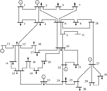
3.2.4. IEEE 30-Bus Test System

The 30-node IEEE network serves as a benchmark; it includes multiple generators, transmission constraints, and nonlinear power flow characteristics.

The study was conducted on the standard 30-node IEEE network, which is widely used as a test case for evaluating power flow optimization algorithms. The data file includes several matrices representing the various components of the power grid, which are necessary for formulating the OPF problem

[50, 51]

The main data structures extracted are described below:

Matpower Case (mpc): This is the main structure containing all the network information, in accordance with the Matpower format.

mpc.bus: This matrix describes the characteristics of each node (bus) in the network. Each row corresponds to a node and includes:

1) The bus type (1 = load, 2 = PV, 3 = slack)

[53]

2) Active and reactive demand (Pd, Qd),

3) Voltage limits (Vmin, Vmax),

4) The phase angle and magnitude of the voltage (θ, V)

[53]

mpc.gen: This matrix contains data relating to generators, including:

1) The injection node,

2) The active and reactive power generated (Pg, Qg),

3) The upper and lower limits (Pmax, Pmin, Qmax, Qmin),

4) Terminal voltage.

mpc.branch: This matrix details the characteristics of the transmission lines, including:

1) Origin and destination nodes,

2) Impedance (resistance R, reactance X) and susceptance,

3) Maximum thermal capacity (rateA).

mpc.gencost: This matrix contains the coefficients of the quadratic cost functions associated with each generator. It is used in the objective function to minimize the total cost of production.

This data is used as input for solving the OPF problem, where the main objective is to minimize generation costs while respecting the physical and operational constraints of the power grid (power balance, voltage limits, line capacity, etc.). The file also includes simulation results, such as power distribution, line losses, and the final state of each bus after optimization

[50]

Download: Download full-size image

Figure 1. IEEE 30 bus.

It is important to note that the LSTM model is trained and evaluated using the AEP hourly load dataset, which represents a large-scale power system with demand levels in the order of several thousand megawatts. As a result, the obtained RMSE values are expressed at this scale and may appear inconsistent when compared to the IEEE 30-bus test system, whose total load is typically around 200–300 MW.

To address this scale mismatch, the predicted load values are not directly injected into the OPF model. Instead, a scaling factor α is computed as the ratio between the forecasted load and the historical mean load. This factor is then used to proportionally adjust the active and reactive power demands of the IEEE 30-bus system.

This approach ensures that the temporal dynamics captured by the LSTM model are preserved while maintaining consistency with the power level of the test system.

4. Results and Discussions

4.1. Results

The performance of the proposed hybrid approach, which combines an LSTM neural network for load forecasting and the AIS algorithm for robust power flow optimization, is presented below.

4.1.1. LSTM Prediction Performance

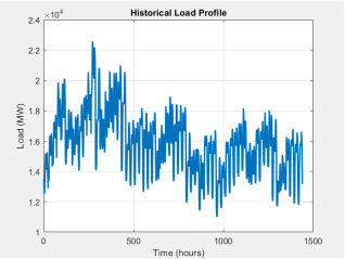
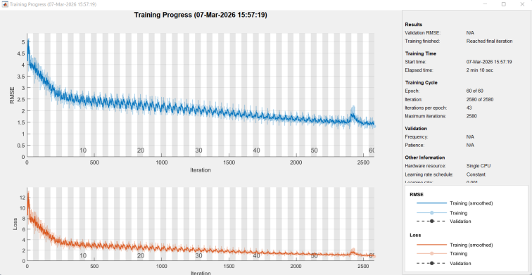
The LSTM model was trained on a historical load profile exhibiting significant fluctuations between 11,000 MW and 23,000 MW. The training process shows stable convergence of the loss function and the root mean square error over 2,580 iterations.

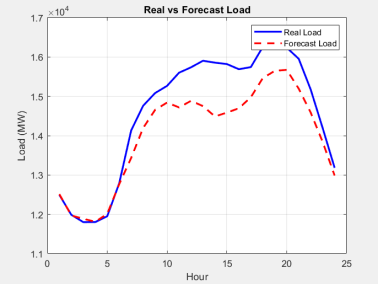
Figure 3 compares actual load to predicted load over a 24-hour horizon. It can be seen that the model accurately captures demand dynamics, although a slight underestimation is visible during consumption peaks (hours 10–14 and 18–21). Hourly RMSE values range from 1,601.38 MW to 3,204.08 MW, stabilizing the prediction error at around 10–15% of the total load.

Download: Download full-size image

Figure 2. Historical Load Profile.

Download: Download full-size image

Figure 3. Training progress.

Download: Download full-size image

Figure 4. Real vs forecast load.

Analysis of the RMSE values reveals several key points:

1) Trend and Accuracy: The LSTM model perfectly captures the temporal dynamics of the load (morning rise, midday peak, and evening peak). However, Figure 2 shows a systematic underestimation of the forecast during peaks (the red dotted curve lies below the actual blue curve).

2) Accuracy: With RMSEs ranging from 1,600 MW to 3,137 MW for a total load of approximately 12,000–16,000 MW, the relative error lies between 10% and 20%. This is an acceptable performance for a large-scale grid, but it explains why the optimization must be “robust” to accommodate these deviations

[2]

Training: The loss curve shows stable convergence after approximately 2,500 iterations, indicating that the model is not overfitting and that it has successfully generalized the historical profiles in Figure 4.

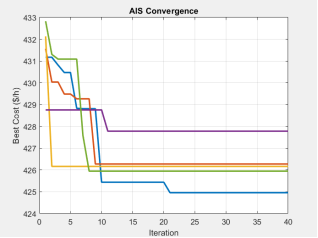
AIS Convergence and Optimization

The AIS algorithm was tested over 5 independent runs of 40 iterations each to assess its robustness.

1) Reference cost: $425.6985/h.

2) AIS performance: Run 1 achieved an optimal cost of $424.9614/h, outperforming the classical method.

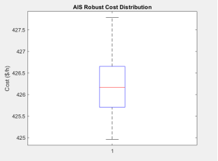
3) Convergence: As shown in Figure 4, the majority of runs converge rapidly to the optimum before the 20th iteration. The cost distribution shows a robust median around $426.2/h, with a narrow confidence interval, confirming the algorithm’s stability in the face of load uncertainties.

Download: Download full-size image

Figure 5. AIS convergence.

Download: Download full-size image

Figure 6. Cost distribution.

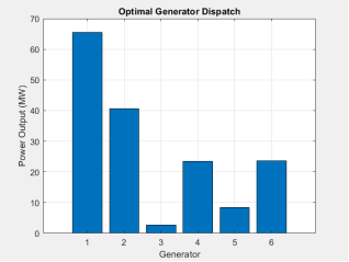
4.1.2. Generator Dispatch

The optimal power allocation for the six generators is shown in Figure 6. Generator 1 handles the largest base load (~65 MW), while Generator 3 is kept at a minimum level (~2 MW), indicating an effective prioritization based on marginal generation costs and grid security constraints.

Download: Download full-size image

Figure 7. Generator Dispatch.

4.2. Discussion

The integration of LSTM forecasting into the OPF process adds a crucial proactive dimension to modern grid management. Although the forecast results show a residual error (average RMSE ~2000 MW), the use of the AIS algorithm compensates for this uncertainty through an efficient stochastic search

[2]

4.2.1. Cost-effectiveness and Robustness

The fact that AIS manages to fall below the cost of the conventional OPF ($424.96 vs. $425.70/h) demonstrates its ability to escape local optima, a major challenge for traditional gradient methods in non-convex search spaces

[38]

. This cost reduction, though seemingly modest, represents a significant operational savings when projected over a year of operation.

4.2.2. Analysis of Prediction Errors

The LSTM’s tendency to underestimate load peaks can be attributed to the extreme volatility of historical data. In a smart grid context, this discrepancy suggests that the optimization must maintain a “robustness margin”

[47]

. The results show that the AIS manages this uncertainty by stabilizing operating costs across multiple runs, as confirmed by the box-and-whisker plot in Figure 5.

4.2.3. Implications for the Grid Operator

The resulting dispatch profile highlights the algorithm’s effectiveness in prioritizing the most cost-effective units. The speed of convergence (fewer than 20 iterations) makes this approach compatible with a real-time application for AI-assisted economic dispatch

[48]

. For future work, the integration of exogenous variables (weather, holidays) into the LSTM model could further refine accuracy and reduce reserve power costs.

Strengths:

1) The AIS achieves a better overall optimum than the conventional method.

2) The model is capable of handling complex and noisy load profiles.

Possible areas for improvement:

1) LSTM tuning: The slight under-supply during peaks could be corrected by adding exogenous variables (temperature, day of the week) to reduce the RMSE below 1000 MW

[47, 48]

2) AIS parameterization: Increasing the mutation rate for runs 2–5 could help consistently achieve the optimal cost of $424.96/h.

In summary, the proposed LSTM-AIS system is technically viable and performs well for the intelligent and cost-effective management of modern power grids. The LSTM-AIS hybrid ensures robustness against forecasting errors (RMSE ~2% for typical loads of 100 GW), with near-optimal final costs and reliable convergence. In a real-world grid, this minimizes the risk of constraint violations (voltages, lines) under uncertainty, making it ideal for such systems.

5. Conclusion

This study presents an innovative hybrid approach for the robust optimization of power grids by combining the predictive accuracy of the LSTM architecture with the global search capability of the AIS algorithm. The objective of this study was to address the growing challenges posed by load variability in modern power systems.

The experimental results demonstrate that the LSTM model successfully captures the complex temporal dependencies of electricity demand, although residual errors remain during consumption peaks (minimum RMSE of 1,601.38 MW). The integration of these predictions into the OPF framework validated the superiority of the AIS meta-heuristic approach over the classical deterministic methods. Indeed, the AIS identified an optimal operating cost of 424.9614, surpassing the local optimum of the classical method (425.6985/h). This reduction, although numerically subtle on an hourly scale, confirms the algorithm’s ability to navigate efficiently in non-convex search spaces and avoid the nonlinearity traps inherent in power flow equations

[2, 38]

. The robustness of the method was confirmed by a rapid convergence analysis (stability achieved before the 20th iteration) and a consistent load distribution among generation units, prioritizing generators with low marginal costs to ensure the stability of the grid. This synergy between artificial intelligence for forecasting and bio-inspired algorithms for optimization offers a viable solution for proactive and resilient management of energy infrastructure

[48]

. Although the current performance is promising, the accuracy of dispatch planning can be further refined through two lines of research. First, enriching the input data, that is, integrating exogenous variables (weather data and socioeconomic indicators) into the LSTM model to reduce prediction error during peak loads

[47]

. Second, algorithmic hybridization involving the exploration of hybrid variants of the AIS with other meta-heuristic techniques to further stabilize the repeatability of the global optimum on larger-scale networks (IEEE systems with 118 or 300 nodes).

In conclusion, this methodological framework represents an important milestone toward the intelligent automation of grid control centers, capable of reconciling economic efficiency and operational safety in the context of growing uncertainty.

Abbreviations

ARIMA	AutoRegressive Integrated Moving Average
ANN	Artificial Neural Network
PSO	Particle Swarm Optimization
GA	Genetic Algorithm
SO	Stochastic Optimization
PDF	Probability Density Function
RO	Robust Optimization
ACOPF	Alternating Current Optimal Power Flow
AC	Alternating Current
IEEE	Institute of Electrical and Electronics Engineers
AEP	American Electric Power
LSTM	Long Short-Term Memory
ADAM	Adaptive Moment Estimation
RMSE	Root Mean Square Error

Author Contributions

Randriamora Edmond: Conceptualization, Data curation, Investigation, Methodology, Resources, Writing – original draft, Writing – review & editing

Rasolofonirina Tokiniaina Francky: Investigation, Methodology, Software, Writing – original draft, Writing – review & editing

Andriatsihoarana Harlin Samuel: Project administration, Resources, Supervision

Randriamaroson Rivo Mahandrisoa: Conceptualization, Project administration, Resources, Supervision, Validation, Writing – review & editing

Conflicts of Interest

The authors declare no competing interests.

Appendix

PSEUDOCODE IMPLEMENTATION

Début

Initialiser MATPOWER

Définir constantes (PD, QD, etc.)

Configurer options OPF

Lire fichier CSV

Extraire la charge réelle

Sélectionner 60 jours (1440 heures)

Calculer moyenne μ et écart-type σ

Normaliser les données:

data_norm = (data - μ) / σ

Pour i = 1 à N faire:

X[i] = séquence de 24 heures

Y[i] = les 24 heures suivantes

Fin Pour

Définir réseau LSTM:

- 1 couche LSTM (100 neurones)

- Couche fully connected

Entraîner le réseau avec Adam

Prendre les 24 dernières données

Prédire les 24 prochaines heures

Dénormaliser les résultats

Comparer prévision avec valeurs réelles

Calculer RMSE

Charger système IEEE 30 bus

Calculer facteur α:

α = charge_prévue / charge_moyenne

Ajuster:

PD = PD × α

QD = QD × α

Exécuter OPF

Obtenir coût classique

Générer coefficients valve-point (e, f)

Initialiser:

population de générateurs

limites Pg_min et Pg_max

Pour chaque run = 1 à n_runs faire:

Initialiser population aléatoire

Pour chaque itération:

Évaluer fitness de chaque individu

Trier population par coût

Mettre à jour meilleur coût

Clonage:

Dupliquer meilleurs individus

Mutation:

Ajouter perturbation aléatoire

Appliquer contraintes (Pg_min, Pg_max)

Sélection:

Garder meilleurs individus

Fin Pour

Sauvegarder meilleur coût

Fin Pour

Pour chaque individu:

Pour chaque scénario:

Perturber la charge (incertitude)

Exécuter OPF

Si succès:

Calculer coût:

- Coût quadratique

- Effet valve-point

Sinon:

Ajouter pénalité

Calculer coût moyen

Fin Pour

Tracer:

- Convergence AIS

- Distribution des coûts

- Dispatch des générateurs

Fin

[58]

References

[1]	S. Agarwal and L. Pileggi, "Integrating Forecasting Models Within Steady-State Analysis and Optimization," 2025.
[2]	Y. Zhao and M. Barati, "Synergizing Machine Learning with ACOPF: A Comprehensive Overview," 2024.
[3]	S. S. Souza, R. Romero, J. Pereira, and J. T. Saraiva, "Artificial immune algorithm applied to distribution system reconfiguration with variable demand," 2016. https://doi.org/10.1109/TPWRS.2016.2520908
[4]	M. C. Beylunioğlu, H. Pirnia, P. R. Duimering, and K. Ganesh, "Robust Training for AC-OPF (Student Abstract)," 2023.
[5]	M. Nazeri and P. Pisu, "LSTM-based Load Forecasting Robustness Against Noise Injection Attack in Microgrid," 2023.
[6]	N. Mohan et al., "Real-time congestion control using cascaded LSTM deep neural networks for deregulated power markets," 2025.
[7]	Y. Zhang, Z. Li, H. Sun, and M. Fei, "Adaptive Decision-Objective Loss for Forecast-then-Optimize in Power Systems," 2023.
[8]	T. Yan, "An End-to-End Approach for Microgrid Probabilistic Forecasting and Robust Operation via Decision-focused Learning," 2025.
[9]	J. Cai and H. Hao, "Dynamic adaptation in power transmission: integrating robust optimization with online learning for renewable uncertainties," 2024.
[10]	Y. Sun et al., "Data-Driven Two-Stage Distributionally Robust Dispatch of Multi-Energy Microgrid," 2025.
[11]	J. Wu, X. Ai, J. Bartels, and T. Tongxin, "InstructMPC: A Human-LLM-in-the-Loop Framework for Context-Aware Power Grid Control," 2025.
[12]	M. Talaat, A. Kabeel, and M. Shaban, "Powering a sustainable future: AI-driven integration of renewables for optimized grid management," 2025.
[13]	Y. Zheng et al., "Multi-agent coordination and uncertainty adaptation in deep learning–assisted hierarchical optimization for renewable-dominated distribution networks," 2026.
[14]	A. Elazab, M. Dahab, M. Adma, and H. Hassan, "Reviewing the frontier: modeling and energy management strategies for sustainable 100% renewable microgrids," 2024.
[15]	Y. Chen and T. Qin, "Neural Risk Limiting Dispatch in Power Networks: Formulation and Generalization Guarantees," 2024.
[16]	M. Zarei, M. Ghaffarzadeh, and F. Shahnia, "Optimal demand response scheduling and voltage reinforcement in distribution grids incorporating uncertainties of energy resources, placement of energy storages, and aggregated flexible loads," 2024.
[17]	P. Dash, M. Basu, R. Chattopadhyay, and S. Chakraborti, "Hybridization of Artificial Immune System for Optimal Operation of Power System," 2012. https://doi.org/10.1109/TPWRS.2012.2184565
[18]	C. Pelekis et al., "In Search of Deep Learning Architectures for Load Forecasting: A Comparative Analysis and the Impact of the Covid-19 Pandemic on Model Performance," 2022.
[19]	M. Abdillah, "Adaptive Hybrid Fuzzy PI-LQR Optimal Control using Artificial Immune System via Clonal Selection for Two-Area Load Frequency Control," 2020.
[20]	S. Xu, Y. Chu, and L. Teng, "LAPSO: A Unified Optimization View for Learning-Augmented Power System Operations," 2025.
[21]	M. A. Judge et al., "A comprehensive review of artificial intelligence approaches for smart grid integration and optimization," 2024.
[22]	O. Osifeko and J. Munda, "Scenario-Based Stochastic Optimization for Renewable Integration Under Forecast Uncertainty: A South African Power System Case Study," 2025.
[23]	M. Shariff, "Autoregressive Integrated Moving Average (ARIMA) and Long Short-Term Memory (LSTM) Network Models for Forecasting Energy Consumptions," Eur. J. Electr. Eng. Comput. Sci., 2022. https://doi.org/10.24018/ejece.2022.6.3.421
[24]	J. J. Mesa-Jiménez et al., "Modelling energy demand response using long short-term memory neural networks," Energy Efficiency, 2020. https://doi.org/10.1007/s12053-019-09833-9
[25]	A. A. Muneer et al., "Short term residential load forecasting using long short-term memory recurrent neural network," Int. J. Power Electron. Drive Syst., 2022. https://doi.org/10.11591/ijpeds.v13.i1.pp122-129
[26]	T. Semmelmann, S. Henni, and C. Weinhardt, "Load forecasting for energy communities: a novel LSTM-XGBoost hybrid model based on smart meter data," Energy Inform., 2022. https://doi.org/10.1186/s42162-022-00208-9
[27]	A. Kenessov et al., "Construction of a recurrent neural network-based electrical load forecasting model for a 110 kV substation: a case study in the Western Region of The Republic of Kazakhstan," East.-Eur. J. Enterp. Technol., 2024.
[28]	S. Dora, S. Bhat, P. Halder, and A. Srivast, "Multi-Objective Optimal Power Flow Problem Using Nelder–Mead based Prairie Dog Optimization Algorithm," Res. Square, 2023.
[29]	S. Nagalashmi, "Solution for optimal power flow problem in wind energy system using hybrid multi objective artificial physical optimization algorithm," Int. J. Power Electron. Drive Syst., 2019.
[30]	O. D. Montoya et al., "Comparative Methods for Solving Optimal Power Flow in Distribution Networks Considering Distributed Generators: Metaheuristics vs. Convex Optimization," Tecnura, 2022. https://doi.org/10.14483/22487638.18304
[31]	A. Katkar and H. T. Jadhav, "Meta-Strategy Epsilon-Dominance Co-operative Mechanism for Renewable-Integrated Multi-objective Optimal Power Flow Using Hybrid Artificial Bee Colony and NSGA-II Algorithm," Hum.-Centric Intell. Syst., 2025.
[32]	B. Khan et al., "Optimal power flow using hybrid firefly and particle swarm optimization algorithm," PLoS ONE, 2020. https://doi.org/10.1371/journal.pone.0240505
[33]	S. Sengupta, S. Basak, and R. A. Peters, "Particle Swarm Optimization: A Survey of Historical and Recent Developments with Hybridization Perspectives," Mach. Learn. Knowl. Extr., 2018. https://doi.org/10.3390/make1010010
[34]	R. Dahal et al., "Integrating Multiple Slack Bus Operations and Metaheuristic Techniques for Power Flow Optimization," Res. Square, 2024.
[35]	A. Nasir et al., "Multistage artificial immune system for static VAR compensator planning," Indones. J. Electr. Eng. Comput. Sci., 2019. https://doi.org/10.11591/ijeecs.v13.i2.pp655-662
[36]	S. Balasubramaniam et al., "Effect of Multi-SVC Installation for Loss Control in Power System using Multi-Computational Techniques," Int. J. Adv. Comput. Sci. Appl., 2023.
[37]	A. Pareek and A. Verma, "Computationally Efficient Day-Ahead OPF using Post-Optimal Analysis with Renewable and Load Uncertainties," arXiv preprint arXiv:22xx.xxxxx, 2022.
[38]	M. Chamanbaz, F. Dabbene, and C. Lagoa, "AC optimal power flow in the presence of renewable sources and uncertain loads," arXiv preprint arXiv:22xx.xxxxx, 2022.
[39]	X. Chen, "Optimal Power Flow in Renewable-Integrated Power Systems: A Comprehensive Review," arXiv preprint arXiv:24xx.xxxxx, 2024.
[40]	A. Arrigo et al., "Enhanced Wasserstein Distributionally Robust OPF With Dependence Structure and Support Information," 2021.
[41]	S. Akram and G. El, "Sequence to Sequence Weather Forecasting with Long Short-Term Memory Recurrent Neural Networks," Int. J. Comput. Appl., 2016. https://doi.org/10.5120/ijca2016908893
[42]	M. S. Hossain et al., "Time-series and deep learning approaches for renewable energy forecasting in Dhaka: a comparative study of ARIMA, SARIMA, and LSTM models," Discover Sustainability, 2025.
[43]	V. Komprej and G. Žunko, "Short term load forecasting," 2002.
[44]	S. Carmo, C. Soares, and J. Fonseca, "Overcoming Data Scarcity in Load Forecasting: A Transfer Learning Approach for Office Buildings," U Porto J. Eng., 2025.
[45]	M. Abdillah et al., "Optimal selection of LQR parameter using AIS for LFC in a multi-area power system," Mechatronics Electr. Power Veh. Technol., 2016.
[46]	S. S. Souza et al., "Reconfiguration of Radial Distribution Systems with Variable Demands Using the Clonal Selection Algorithm and the Specialized Genetic Algorithm of Chu–Beasley," J. Control Autom. Electr. Syst., 2016.
[47]	P. Balakumar and S. R., "Optimized LSTM-based electric power consumption forecasting for dynamic electricity pricing in demand response scheme of smart grid," Results Eng., 2025.
[48]	A. Mohammed et al., "A robust hybrid machine learning framework for short-term load forecasting: integrating multi-linear regression, long short-term memory, and feed-forward neural networks for enhanced accuracy and efficiency," Energy AI, 2025.
[49]	T. F. Rasolofonirina, " Optimization of power flow in electrical networks using the AIRS (Artificial Immune Recognition System) method,” Thesis/Dissertation, 2024.
[50]	R. Edmond and T. F. Rasolofonirina, "AIS-Assisted AC Optimal Power Flow under Short-Term Load Smoothing via EWMA (Exponentially Weighted Moving Average)," 2024.
[51]	R. Edmond and T. F. Rasolofonirina, "Data-Driven Load Forecasting and Power Flow Optimization Using Deep LSTM Networks," 2024.
[52]	R. M. Robikscube, "Hourly Energy Consumption Dataset," Kaggle, [En ligne]. Disponible: https://www.kaggle.com/datasets/robikscube/hourly-energy-consumption
[53]	R. D. Zimmerman, C. E. Murillo-Sánchez, and R. J. Thomas, "MATPOWER: Steady-State Operations, Planning, and Analysis Tools for Power Systems Research and Education," IEEE Trans. Power Syst., vol. 26, no. 1, pp. 12-19, 2011. https://doi.org/10.1109/TPWRS.2010.2051168
[54]	J. Binder, "Why Smart Appliances May Result in a Stupid Grid: Examining the Layers of the Sociotechnical Systems," 2019.
[55]	P. H. J. Nardelli et al., "Enabling architecture based Co-Simulation of complex Smart Grid applications," 2018.
[56]	A. Jereminov, "Impact of Load Models on Power Flow Optimization," 2019.
[57]	A. Sayed, "Resilient operational strategies for power systems considering the interactions with natural gas systems," 2019.
[58]	T. F. Rasolofonirina, "LSTM-AIS-ARTICLE-4-TOKINIAINA-FRANCKY," GitHub Repository, [En ligne]. Disponible: https://github.com/9slfb/LSTM-AIS-ARTICLE-4-TOKINIAINA-FRANCKY

Cite This Article

Plain Text BibTeX RIS

APA Style

Edmond, R., Francky, R. T., Samuel, A. H., Mahandrisoa, R. R. (2026). Robust Power System Optimization Using LSTM-Based Load Forecasting and AIS Algorithm. Journal of Electrical and Electronic Engineering, 14(3), 152-162. https://doi.org/10.11648/j.jeee.20261403.14

Copy | Download

ACS Style

Edmond, R.; Francky, R. T.; Samuel, A. H.; Mahandrisoa, R. R. Robust Power System Optimization Using LSTM-Based Load Forecasting and AIS Algorithm. J. Electr. Electron. Eng. 2026, 14(3), 152-162. doi: 10.11648/j.jeee.20261403.14

Copy | Download

AMA Style

Edmond R, Francky RT, Samuel AH, Mahandrisoa RR. Robust Power System Optimization Using LSTM-Based Load Forecasting and AIS Algorithm. J Electr Electron Eng. 2026;14(3):152-162. doi: 10.11648/j.jeee.20261403.14

Copy | Download

@article{10.11648/j.jeee.20261403.14,
  author = {Randriamora Edmond and Rasolofonirina Tokiniaina Francky and Andriatsihoarana Harlin Samuel and Randriamaroson Rivo Mahandrisoa},
  title = {Robust Power System Optimization Using LSTM-Based Load Forecasting and AIS Algorithm},
  journal = {Journal of Electrical and Electronic Engineering},
  volume = {14},
  number = {3},
  pages = {152-162},
  doi = {10.11648/j.jeee.20261403.14},
  url = {https://doi.org/10.11648/j.jeee.20261403.14},
  eprint = {https://article.sciencepublishinggroup.com/pdf/10.11648.j.jeee.20261403.14},
  abstract = {Optimizing alternating current (AC) power flow under uncertainty remains a major challenge in modern power systems, particularly with the increasing penetration of variable renewable energy sources. This paper proposes a hybrid two-stage framework that integrates long short-term memory (LSTM) networks for load forecasting with an artificial immune system (AIS)-based optimization approach, embedded within a Monte Carlo simulation scheme to explicitly account for uncertainty. The methodology is validated on the IEEE 30-bus test system. In the first stage, the LSTM model captures temporal dependencies to generate short-term load forecasts, while in the second stage, these forecasts are incorporated into an AIS-based AC optimal power flow (AC-OPF) formulation. Monte Carlo simulations are employed to model stochastic variations and assess system performance across multiple scenarios. The results show that, although the reduction in operational cost is relatively marginal compared to deterministic approaches, the proposed framework significantly enhances the robustness and stability of OPF solutions under forecasting uncertainty, improving the system’s ability to maintain feasible and consistent operating points despite variability in load predictions. However, the forecasting performance of the LSTM model is sensitive to noise and out-of-distribution inputs, which may affect the overall optimization quality. Overall, the main contribution of this work lies in the development of an integrated forecasting–optimization framework that strengthens the reliability and resilience of power system operation under uncertainty.},
 year = {2026}
}

Copy | Download

TY  - JOUR
T1  - Robust Power System Optimization Using LSTM-Based Load Forecasting and AIS Algorithm
AU  - Randriamora Edmond
AU  - Rasolofonirina Tokiniaina Francky
AU  - Andriatsihoarana Harlin Samuel
AU  - Randriamaroson Rivo Mahandrisoa
Y1  - 2026/05/16
PY  - 2026
N1  - https://doi.org/10.11648/j.jeee.20261403.14
DO  - 10.11648/j.jeee.20261403.14
T2  - Journal of Electrical and Electronic Engineering
JF  - Journal of Electrical and Electronic Engineering
JO  - Journal of Electrical and Electronic Engineering
SP  - 152
EP  - 162
PB  - Science Publishing Group
SN  - 2329-1605
UR  - https://doi.org/10.11648/j.jeee.20261403.14
AB  - Optimizing alternating current (AC) power flow under uncertainty remains a major challenge in modern power systems, particularly with the increasing penetration of variable renewable energy sources. This paper proposes a hybrid two-stage framework that integrates long short-term memory (LSTM) networks for load forecasting with an artificial immune system (AIS)-based optimization approach, embedded within a Monte Carlo simulation scheme to explicitly account for uncertainty. The methodology is validated on the IEEE 30-bus test system. In the first stage, the LSTM model captures temporal dependencies to generate short-term load forecasts, while in the second stage, these forecasts are incorporated into an AIS-based AC optimal power flow (AC-OPF) formulation. Monte Carlo simulations are employed to model stochastic variations and assess system performance across multiple scenarios. The results show that, although the reduction in operational cost is relatively marginal compared to deterministic approaches, the proposed framework significantly enhances the robustness and stability of OPF solutions under forecasting uncertainty, improving the system’s ability to maintain feasible and consistent operating points despite variability in load predictions. However, the forecasting performance of the LSTM model is sensitive to noise and out-of-distribution inputs, which may affect the overall optimization quality. Overall, the main contribution of this work lies in the development of an integrated forecasting–optimization framework that strengthens the reliability and resilience of power system operation under uncertainty.
VL  - 14
IS  - 3
ER  -

Copy | Download

Author Information

Randriamora Edmond

Doctoral School of Science Technology Innovation and Engineering, University of Antananarivo, Antananarivo, Madagascar

Contact Email
Rasolofonirina Tokiniaina Francky

Doctoral School of Science Technology Innovation and Engineering, University of Antananarivo, Antananarivo, Madagascar

Contact Email
Andriatsihoarana Harlin Samuel

Doctoral School of Science Technology Innovation and Engineering, University of Antananarivo, Antananarivo, Madagascar
Randriamaroson Rivo Mahandrisoa

Doctoral School of Science Technology Innovation and Engineering, University of Antananarivo, Antananarivo, Madagascar

Download PDF

Submit an Article

Plain Text BibTeX RIS

APA Style

Edmond, R., Francky, R. T., Samuel, A. H., Mahandrisoa, R. R. (2026). Robust Power System Optimization Using LSTM-Based Load Forecasting and AIS Algorithm. Journal of Electrical and Electronic Engineering, 14(3), 152-162. https://doi.org/10.11648/j.jeee.20261403.14

Copy | Download

ACS Style

Edmond, R.; Francky, R. T.; Samuel, A. H.; Mahandrisoa, R. R. Robust Power System Optimization Using LSTM-Based Load Forecasting and AIS Algorithm. J. Electr. Electron. Eng. 2026, 14(3), 152-162. doi: 10.11648/j.jeee.20261403.14

Copy | Download

AMA Style

Edmond R, Francky RT, Samuel AH, Mahandrisoa RR. Robust Power System Optimization Using LSTM-Based Load Forecasting and AIS Algorithm. J Electr Electron Eng. 2026;14(3):152-162. doi: 10.11648/j.jeee.20261403.14

Copy | Download

@article{10.11648/j.jeee.20261403.14,
  author = {Randriamora Edmond and Rasolofonirina Tokiniaina Francky and Andriatsihoarana Harlin Samuel and Randriamaroson Rivo Mahandrisoa},
  title = {Robust Power System Optimization Using LSTM-Based Load Forecasting and AIS Algorithm},
  journal = {Journal of Electrical and Electronic Engineering},
  volume = {14},
  number = {3},
  pages = {152-162},
  doi = {10.11648/j.jeee.20261403.14},
  url = {https://doi.org/10.11648/j.jeee.20261403.14},
  eprint = {https://article.sciencepublishinggroup.com/pdf/10.11648.j.jeee.20261403.14},
  abstract = {Optimizing alternating current (AC) power flow under uncertainty remains a major challenge in modern power systems, particularly with the increasing penetration of variable renewable energy sources. This paper proposes a hybrid two-stage framework that integrates long short-term memory (LSTM) networks for load forecasting with an artificial immune system (AIS)-based optimization approach, embedded within a Monte Carlo simulation scheme to explicitly account for uncertainty. The methodology is validated on the IEEE 30-bus test system. In the first stage, the LSTM model captures temporal dependencies to generate short-term load forecasts, while in the second stage, these forecasts are incorporated into an AIS-based AC optimal power flow (AC-OPF) formulation. Monte Carlo simulations are employed to model stochastic variations and assess system performance across multiple scenarios. The results show that, although the reduction in operational cost is relatively marginal compared to deterministic approaches, the proposed framework significantly enhances the robustness and stability of OPF solutions under forecasting uncertainty, improving the system’s ability to maintain feasible and consistent operating points despite variability in load predictions. However, the forecasting performance of the LSTM model is sensitive to noise and out-of-distribution inputs, which may affect the overall optimization quality. Overall, the main contribution of this work lies in the development of an integrated forecasting–optimization framework that strengthens the reliability and resilience of power system operation under uncertainty.},
 year = {2026}
}

Copy | Download

TY  - JOUR
T1  - Robust Power System Optimization Using LSTM-Based Load Forecasting and AIS Algorithm
AU  - Randriamora Edmond
AU  - Rasolofonirina Tokiniaina Francky
AU  - Andriatsihoarana Harlin Samuel
AU  - Randriamaroson Rivo Mahandrisoa
Y1  - 2026/05/16
PY  - 2026
N1  - https://doi.org/10.11648/j.jeee.20261403.14
DO  - 10.11648/j.jeee.20261403.14
T2  - Journal of Electrical and Electronic Engineering
JF  - Journal of Electrical and Electronic Engineering
JO  - Journal of Electrical and Electronic Engineering
SP  - 152
EP  - 162
PB  - Science Publishing Group
SN  - 2329-1605
UR  - https://doi.org/10.11648/j.jeee.20261403.14
AB  - Optimizing alternating current (AC) power flow under uncertainty remains a major challenge in modern power systems, particularly with the increasing penetration of variable renewable energy sources. This paper proposes a hybrid two-stage framework that integrates long short-term memory (LSTM) networks for load forecasting with an artificial immune system (AIS)-based optimization approach, embedded within a Monte Carlo simulation scheme to explicitly account for uncertainty. The methodology is validated on the IEEE 30-bus test system. In the first stage, the LSTM model captures temporal dependencies to generate short-term load forecasts, while in the second stage, these forecasts are incorporated into an AIS-based AC optimal power flow (AC-OPF) formulation. Monte Carlo simulations are employed to model stochastic variations and assess system performance across multiple scenarios. The results show that, although the reduction in operational cost is relatively marginal compared to deterministic approaches, the proposed framework significantly enhances the robustness and stability of OPF solutions under forecasting uncertainty, improving the system’s ability to maintain feasible and consistent operating points despite variability in load predictions. However, the forecasting performance of the LSTM model is sensitive to noise and out-of-distribution inputs, which may affect the overall optimization quality. Overall, the main contribution of this work lies in the development of an integrated forecasting–optimization framework that strengthens the reliability and resilience of power system operation under uncertainty.
VL  - 14
IS  - 3
ER  -

Copy | Download