Probabilistic and stochastic models such as Bayesian and Hidden Markov models can cope well with system uncertainties, but there is a problem of how learning state prediction and learning path generation are performed independently and how to connect them, and the overall effect of the system may be lost even after the connection. Using a Markov Decision Process, a kind of reinforcement learning model, not only can the prediction of the learning state of a student and the generation of a path be implemented simultaneously in a single model, but also the overall error can be reduced. In this paper, we propose to build an intelligent tutoring system into a Markov Decision Process model, an reinforcement learning model, with the aim of reducing learning path generation error and improving system performance by using Markov decision Process model in intelligent tutoring system. In addition, we propose a learning state evaluation method using a Markov Decision Process model to simultaneously proceed the student’s learning state estimation and the system’s action selection. We also propose a method to apply the value-iteration algorithm to action selection computation in a Markov Decision Process model. Comparison with previous models was carried out and its effectiveness was verified.
| Published in | Science Research (Volume 14, Issue 1) |
| DOI | 10.11648/j.sr.20261401.11 |
| Page(s) | 1-13 |
| Creative Commons |
This is an Open Access article, distributed under the terms of the Creative Commons Attribution 4.0 International License (http://creativecommons.org/licenses/by/4.0/), which permits unrestricted use, distribution and reproduction in any medium or format, provided the original work is properly cited. |
| Copyright |
Copyright © The Author(s), 2026. Published by Science Publishing Group |
Reinforcement Learning, MDP, Learning Path Generation
 vector equal to a, and the vector space is divided into different regions.
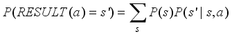
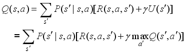
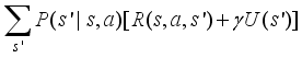
 (1)
(1) 
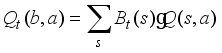 (2)
(2)  is a linear combination of
  for each hidden state with the corresponding confidence level
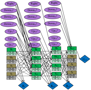
  . When this process converges, taking the optimal action a at time t associated with the largest
  , we obtain π*.
 St-1 | P(St | St-1) | ||
|---|---|---|---|
H | M | L | |
H | 0.85 | 0.1 | 0.05 |
M | 0.3 | 0.4 | 0.3 |
L | 0.1 | 0.4 | 0.5 |
St-1 | P(S1t|St-1) = 0.91 | P(S2t|St-1)=0.03 | P(S3t|St-1)=0.03 | P(S4t|St-1)=0.03 | ||||||||
|---|---|---|---|---|---|---|---|---|---|---|---|---|
H | M | L | H | M | L | H | M | L | H | M | L | |
H | 0.91×0.85 | 0.91×0.1 | 0.91×0.05 | 0.03×0.85 | 0.03×0.1 | 0.03×0.05 | 0.03×0.85 | 0.03×0.1 | 0.03×0.05 | 0.03×0.85 | 0.03×0.1 | 0.03×0.05 |
M | 0.91×0.3 | 0.91×0.4 | 0.91×0.3 | 0.03×0.3 | 0.03×0.4 | 0.03×0.3 | 0.03×0.3 | 0.03×0.4 | 0.03×0.3 | 0.03×0.3 | 0.03×0.4 | 0.03×0.3 |
L | 0.91×0.1 | 0.91×0.4 | 0.91×0.5 | 0.03×0.1 | 0.03×0.4 | 0.03×0.5 | 0.03×0.1 | 0.03×0.4 | 0.03×0.5 | 0.03×0.1 | 0.03×0.4 | 0.03×0.5 |
 (3)
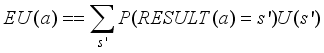
(3)  (4)
(4)  .
. 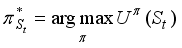 (5)
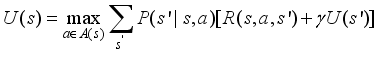
(5)  also recommends some action for every state as a policy, especially if St is an initial state, then it is an optimal policy for the initial state. The use of continuous results of utility values at infinite limits makes the optimal policy independent of the initial state. Of course, the action sequence is not independent of the initial state, but the policy is a function that indicates the action in each state. In the future, we simply denote the optimal strategy by
  .
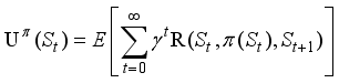
.  . That is,
  is the sum of the expected discount rewards when the intelligent tutoring system executes some optimal policy. This is simply denoted U (St).
 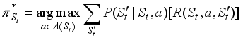 (6)
(6)  (7)
(7)  ,
,  ,
,  , and
, and  .
.  (8)
(8)  (9)
(9)  (10)
(10) 
 (11)
(11) pretest mean (M) | pretest standard deviation (SD) | final test mean (M) | final test standard deviation (SD) | |
|---|---|---|---|---|
Bayesian Model | 6.54 | 1.85 | 6.57 | 1.41 |
MDP | 7.55 | 1.75 | 8.27 | 1.49 |
HMM | 7 | 1.84 | 7.32 | 1.66 |
policy | Pre-test | Post-test | ||||
|---|---|---|---|---|---|---|
overall | fast | slow | overall | fast | slow | |
MDP | 74.90(26.3) | 75.34(27.6) | 74.48(25.5) | 88.26(15.2) | 84.23(17.7) | 92.12(11.3) |
POMDP | 75.18(25.9) | 74.01(29.1) | 76.15(23.2) | 79.53(24.4) | 86.47(23.6) | 73.86(24.1) |
random | 65.99(28.1) | 67.69(28.8) | 64.02(27.8) | 82.85(22.3) | 88.98(17.9) | 75.69(25.3) |
MDP | Markov Decision Process |
POMDP | Partially Observable Markov Decision Process |
MEU | Maximum Expected Utility |
IOHMM | Input-Output Hidden Markov Model |
DBN | Dynamic Bayesian Network |
DDN | Dynamic Decision Network |
S | Slides |
Co | Comments |
V | Videos |
QA | Questions and Answers |
LP | Learning Path |
H | High |
M | Medium |
L | Low |
HMM | Hidden Markov Model |
M | Means |
SD | Standard Deviations |
| [1] |
Russell, S. J., & Norvig, P. (2022). Artificial Intelligence: A Modern Approach. Prentice Hall. Retrieved from
http://www.amazon.com/Artificial-Intelligence-ApproachStuart-Russell/dp/0131038052 |
| [2] | Burhan Aji S. (2022). Intelligent Tutoring System Design Using Markov Decision Process. Emerging Information Science and Technology. Vol. 3, No. 1, pp. 1 9-28. |
| [3] | Iglesias, A., Martinez, P. and Fernandez, F. (2003). An experience applying reinforcement learning in a web-based adaptive and intelligent educational system. Informatics in Education. vol. 2, no. 2, pp. 223-240. |
| [4] | Litman, A. J. and Silliman, S. (2004). Itspoke: An intelligent tutoring spoken dialogue system. in Proc. Human Language Technology Conference 2004. |
| [5] | Sarma, B., and Ravindran, B. (2007). Intelligent tutoring systems using reinforcement learning to teach autistic students. Home Informatics and Telematics: ICT for The Next Billion, Springer, vol. 241, pp. 65-78. |
| [6] | Iglesias, A., Martnez, P., and Fernndez, F. (2009). Learning teaching strategies in an Adaptive and Intelligent Educational System through Reinforcement Learning. Journal Applied Intelligence, Volume 31 Issue 1, August 2009. 58. |
| [7] | Ai, H., Litman, D. J., Forb es-Riley, K., Rotaru, M., Tetreault, J., and Purandare, A. (2006). Using system and user performance features to improve emotion detection in sp oken tutoring dialogs. In Proceedings of the International Conference on Spoken Language Processing (Interspeech 2006 (ICSLP), pages 797–800, Pittsburgh. |
| [8] | Janarthanam, S., Hastie, H., Lemon, O., and Liu, X. (2011). The day after the day after tomorrow: a machine learning approach to adaptive temporal expression generation: training and evaluation with real users. SIGDIAL ’11 Proceedings of the SIGDIAL 2011 Conference (Pages 142-151), Stroudsburg, PA, USA 2011. |
| [9] | Pan, Y. Lee, H., and Lee, L. (2012). Interactive Spoken Document Retrieval With Suggested Key Terms Ranked by a Markov Decision Process. IEEE Transactions on Audio, Speech, and Language Processing archive Volume 20 Issue 2, February 2012, Page 632-645. |
| [10] | Chi, M., Lehn, K., Litman, D., and Jordan, P. (2011). Empirically evaluating the application of reinforcement learning to the induction of effective and adaptive pedagogical strategies. User Model User-Adap, Kluwer Academic, pp. 137-180. |
| [11] | Iglesias, A., Martnez, P., Aler, R., and Fernndez, F. (2009). Learning teaching strategies in an adaptive and intelligent educational system through reinforcement learning. Applied Intelligence, vol. 31, no. 1, pp. 89-106. |
| [12] | Williams, J. D., and Young, S. (2007). Partially observable Markov decision processes for spoken dialog systems. Elsevier Computer Speech and Language, vol. 21, pp. 393-422. |
| [13] | Theocharous, G., Beckwith, R., Butko, N., and Philipose, M. (2009). Tractable POMDP planning algorithms for optimal teaching in SPAIS. in Proc. IJCAI PAIR Workshop 2009. |
| [14] | Rafferty, A. N. et al. (2011). Faster teaching by POMDP planning. in Proc. Artificial Intelligence in Education (AIED) 2011, pp. 280-287. |
| [15] | Chinaei, H. R., Chaib-draa, B., and Lamontagne, L. (2012). Learning observation models for dialogue POMDPs. Canadian AI’12 Proceedings of the 25th Canadian Conference on Advances in Artificial Intelligence, Springer-Verlag Berlin, Heidelberg, pp. 280-286. |
| [16] | Folsom-Kovarik, J. T., Sukthankar, G., and Schatz, S. (2013). Tractable POMDP representations for intelligent tutoring systems. ACM Transactions on Intelligent Systems and Technology (TIST) -Special Section on Agent Communication, Trust in Multiagent Systems, Intelligent Tutoring and Coaching Systems Archive, vol. 4, no. 2, p. 29. |
| [17] | Julien Seznec. (2020). Sequential machine learning for intelligent tutoring systems. Machine Learning [cs.LG]. Université de Lille, 2020. English. ffNT: LILUI084ff ffel-03490620f |
| [18] | Whiteley, W. (2005). Artificially Intelligent Adaptive Tutoring System, Education, IEE Transactions on, Volume 48, Issue 4. |
| [19] | Jeremiah, T. F., Gita, S., and Sae, S. (2013). Tractable POMDP representations or intelligent tutoring systems. ACM Transactions on Intelligent Systems and Technology (TIST) - Special section on agent communication, trust in multiagent ystems, intelligent tutoring and coaching systems archive, Volume 4 Issue 2, March 2013. |
| [20] | Wang, F. (2018). Reinforcement Learning in a POMDP Based Intelligent Tutoring System for Optimizing Teaching Strategies. International Journal of Information and Education Technology, Vol. 8, No. 8, August 2018, pp 553-558. |
| [21] | Hamid, R. C., Brahim, C., Luc, L. (2012). Learning observation models for dialogue POMDPs. Canadian AI’12 Proceedings of the 25th Canadian conference on Advances in Artificial Intelligence, Pages 280-286, Springer-Verlag Berlin, Heidelberg 2012. |
| [22] | Shen, S. (2020). Empirically Evaluating the Effectiveness of POMDP vs. MDP Towards the Pedagogical Strategies Induction, AIED 2020, LNAI 10948, pp. 109–113. |
| [23] | Li, J., and Hou, L. (2017). Review of knowledge graph research. J. Shanxi Univ., Natural Sci. Ed., vol. 40, no. 3, pp. 454–459, Mar. |
| [24] | Chen, Z. et al. (2020). Knowledge Graph Completion: A Review. IEEE Access, 2020.3030076, VOLUME 8. |
APA Style
Kwon, S., Rim, J., Ko, C., Ryu, U., Pak, Y., et al. (2026). Learning Path Generation of ITS Using Markov Decision Process. Science Research, 14(1), 1-13. https://doi.org/10.11648/j.sr.20261401.11
ACS Style
Kwon, S.; Rim, J.; Ko, C.; Ryu, U.; Pak, Y., et al. Learning Path Generation of ITS Using Markov Decision Process. Sci. Res. 2026, 14(1), 1-13. doi: 10.11648/j.sr.20261401.11
AMA Style
Kwon S, Rim J, Ko C, Ryu U, Pak Y, et al. Learning Path Generation of ITS Using Markov Decision Process. Sci Res. 2026;14(1):1-13. doi: 10.11648/j.sr.20261401.11
@article{10.11648/j.sr.20261401.11,
  author = {Song-Hwan Kwon and Jong-Nam Rim and Chung-Song Ko and Un-Song Ryu and Yong-Jin Pak and Hyon-Il Son},
  title = {Learning Path Generation of ITS Using Markov Decision Process},
  journal = {Science Research},
  volume = {14},
  number = {1},
  pages = {1-13},
  doi = {10.11648/j.sr.20261401.11},
  url = {https://doi.org/10.11648/j.sr.20261401.11},
  eprint = {https://article.sciencepublishinggroup.com/pdf/10.11648.j.sr.20261401.11},
  abstract = {Probabilistic and stochastic models such as Bayesian and Hidden Markov models can cope well with system uncertainties, but there is a problem of how learning state prediction and learning path generation are performed independently and how to connect them, and the overall effect of the system may be lost even after the connection. Using a Markov Decision Process, a kind of reinforcement learning model, not only can the prediction of the learning state of a student and the generation of a path be implemented simultaneously in a single model, but also the overall error can be reduced. In this paper, we propose to build an intelligent tutoring system into a Markov Decision Process model, an reinforcement learning model, with the aim of reducing learning path generation error and improving system performance by using Markov decision Process model in intelligent tutoring system. In addition, we propose a learning state evaluation method using a Markov Decision Process model to simultaneously proceed the student’s learning state estimation and the system’s action selection. We also propose a method to apply the value-iteration algorithm to action selection computation in a Markov Decision Process model. Comparison with previous models was carried out and its effectiveness was verified.},
 year = {2026}
}
TY  - JOUR
T1  - Learning Path Generation of ITS Using Markov Decision Process
AU  - Song-Hwan Kwon
AU  - Jong-Nam Rim
AU  - Chung-Song Ko
AU  - Un-Song Ryu
AU  - Yong-Jin Pak
AU  - Hyon-Il Son
Y1  - 2026/01/30
PY  - 2026
N1  - https://doi.org/10.11648/j.sr.20261401.11
DO  - 10.11648/j.sr.20261401.11
T2  - Science Research
JF  - Science Research
JO  - Science Research
SP  - 1
EP  - 13
PB  - Science Publishing Group
SN  - 2329-0927
UR  - https://doi.org/10.11648/j.sr.20261401.11
AB  - Probabilistic and stochastic models such as Bayesian and Hidden Markov models can cope well with system uncertainties, but there is a problem of how learning state prediction and learning path generation are performed independently and how to connect them, and the overall effect of the system may be lost even after the connection. Using a Markov Decision Process, a kind of reinforcement learning model, not only can the prediction of the learning state of a student and the generation of a path be implemented simultaneously in a single model, but also the overall error can be reduced. In this paper, we propose to build an intelligent tutoring system into a Markov Decision Process model, an reinforcement learning model, with the aim of reducing learning path generation error and improving system performance by using Markov decision Process model in intelligent tutoring system. In addition, we propose a learning state evaluation method using a Markov Decision Process model to simultaneously proceed the student’s learning state estimation and the system’s action selection. We also propose a method to apply the value-iteration algorithm to action selection computation in a Markov Decision Process model. Comparison with previous models was carried out and its effectiveness was verified.
VL  - 14
IS  - 1
ER  -
Department of Information Science, University of Science, Pyongyang, Democratic People’s Republic of Korea
Information